Note 32. Designing FIR Filters: Background and Options

The block diagram in Figure 32.1 represents the canonical form for an Mth order finite-impulse response (FIR) digital filter in that the diagram is a direct implementation of the filter’s defining difference equation:

32.1

Figure 32.1. Block diagram for FIR filter

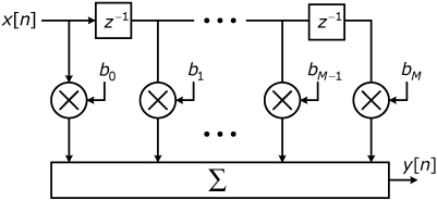
Examination of the equation reveals that the filter’s output at time n is simply a weighted sum of the inputs at times n – M through n. The notation used in Eq. (32.1) is consistent with the notation used in the difference equation for an IIR filter, as presented in Note 49. Comparison of Eqs. (32.1) and (49.1) reveals that FIR filters can be viewed as a special case of IIR filters.

Equation (32.1) has the form of an (M+1)-point discrete convolution, with the coefficients b_k taking the place of the unit-sample-response sequence, h[k]. Therefore, for an FIR filter, the unit sample response, h[k], is defined by the coefficients b_k, and Eq. (32.1) can be immediately rewritten as the convolution equation:

The filter’s system function, H(z), is obtained by taking the z transform of h[k]:

32.2

This system function has zeros but no finite poles, so in some contexts, FIR filters are referred to as all-zero filters. (See Note 44 for a discussion of the z transform.)

32.1. Implementation Structures

The block diagram in Figure 32.1 can be converted into the corresponding signal flow graph shown in Figure 32.2(a). The transposition theorem can be applied to this direct form structure to obtain the transposed direct form structure in Figure 32.2(b).

Figure 32.2. Structures for an FIR filter: (a) direct form, (b) transposed direct form

The system function from Eq. (32.2) can be expressed as a product of first- and second-order polynomials in the form

32.3

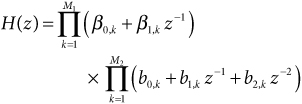
where

m = M₁ + 2M₂

and

• Each real root of H(z) is the root of one of the first-order polynomials.

• Each second-order polynomial has as its roots a complex-conjugate pair of complex roots from H(z).

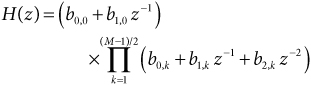
Typical FIR filters usually have a single real root, and for real-input-real-output FIR filters, the complex roots of H(z) always occur in conjugate pairs. Under these constraints, Eq. (32.3) can be rewritten for even M as

32.4

and for odd M as

32.5

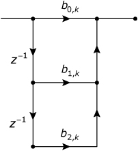
FIR filters can be implemented in a form that mimics the structure of Eq. (32.4) or (32.5). Each second-order polynomial has a complex-conjugate pair of roots and can be implemented as a second-order filter section having real-valued coefficients. The second-order section, shown in Figure 32.3 implements the polynomial

b_{0, k} + b_{1, k} z^–1 + b_{2, k} z^–2

Figure 32.3. A second-order filter section

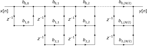
An even-order filter can be implemented as a cascade of these second-order sections, as shown in Figure 32.4. An odd-order filter can be implemented as a cascade of second-order sections plus one first-order section, as shown in Figure 32.5.

Figure 32.4. Cascade structure for an even-length FIR filter

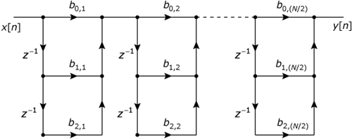
Figure 32.5. Cascade structure for an odd-length FIR filter

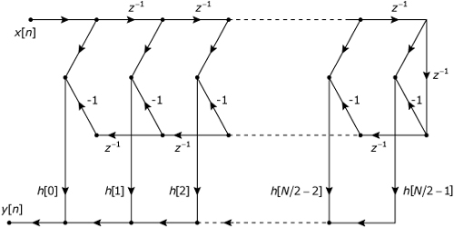
The linear-phase FIR filters discussed in Note 33 all exhibit symmetries in their unit-sample responses. These symmetries, which are listed in Table 32.1, can be exploited to design the efficient implementation structures shown in Figures 32.6 through 32.9.

Table 32.1. Linear-phase FIR Filter Types

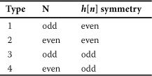
Figure 32.6. Direct-waveform structure for type 1 (odd length, even symmetry) linear-phase FIR filter

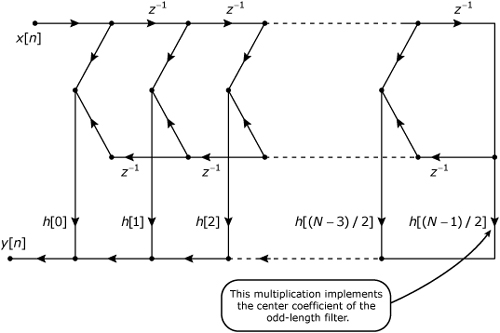
Figure 32.7. Direct-form structure for type 2 (even length, even symmetry) linear-phase FIR filter

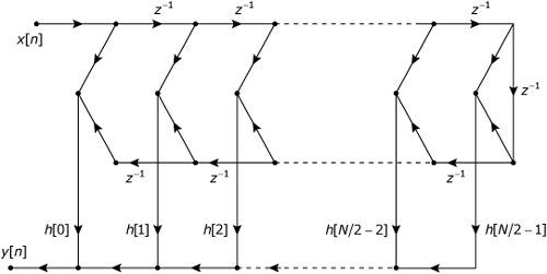
Figure 32.8. Direct-form structure for type 3 (odd length, odd symmetry) linear-phase FIR filter

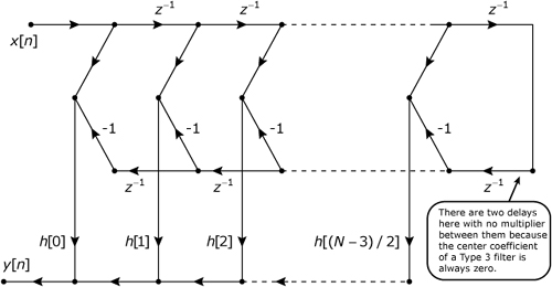
Figure 32.9. Direct-form structure for type 4 (even length, odd symmetry) linear-phase FIR filter