Note 39. Characterizing Analog Filters

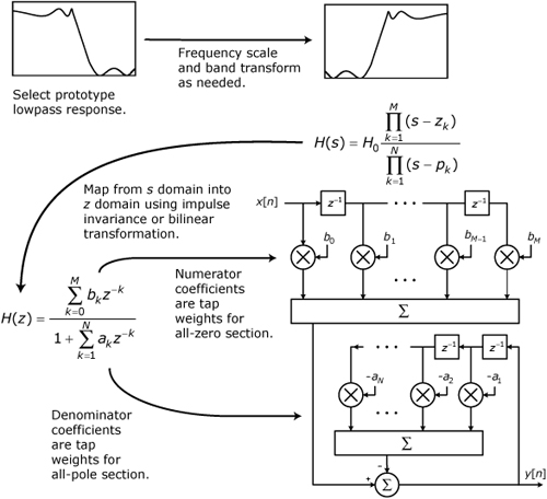
Several of the most popular techniques for designing IIR filters are based on transformations or mappings of analog prototype filters into digital filters. Often these prototype filters are classic filter designs such as Butterworth, Chebyshev, or elliptic. These classical filters are usually presented in the literature as normalized lowpass filters that must be denormalized and possibly transformed into other band configurations before they can be used as protoypes for IIR filters. This note covers techniques that are used to characterize and frequency-scale classical analog filters.

Neglecting imperfections in the components used to implement them, classical analog filters are considered to be time-invariant, lumped-parameter linear systems. The fundamental properties of linear systems are defined in Math Box 39.1.

A linear system can be characterized by a differential equation, step response, impulse response, complex-frequency-domain system function, or transfer function: There are a number of useful and well known relationships between these various characterizations.

• The time-domain input signal, x(t), and output signal, y(t), are related by a time-domain differential equation.

• The complex-frequency-domain system function is obtained by performing the Laplace transform on the time-domain differential equation.

• The impulse response, h(t), can be obtained by solving the differential equation for x(t) set equal to the unit impulse, δ(t).

• The step response, a(t), can be obtained by solving the differential equation for x(t) set equal to the unit step, u(t).

• The impulse response, h(t), can be obtained by differentiating the step response, a(t), with respect to time.

• The step response, a(t), can be obtained by integrating the impulse response, h(t), with respect to time.

• The transfer function can be obtained by solving the complex-frequency-domain system function for H(s) = Y(s)/X(s), where Y(s) and X(s) are, respectively, the Laplace transforms of y(t) and x(t).

• The transfer function, H(s), can be obtained as the Laplace transform of the impulse response, h(t).

39.1. Transfer Functions

The transfer function, H(s), of a system is equal to the Laplace transform of the output signal divided by the Laplace transform of the corresponding input signal:

The transfer function can be put into the form

where P(s) and Q(s) are polynomials in s, and H₀ is the gain of the filter at zero frequency. These polynomials can be expressed in sum-of-powers form to yield

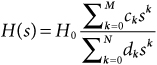
Alternatively, the polynomials P(s) and Q(s) can be expressed in factored form to yield

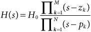
The roots z₁, z₂, . . ., z_M of P(s) are called zeros of the transfer function, and the roots p₁, p₂, . . ., p_N of Q(s) are called poles of the transfer function. For the system represented by H(s) to be stable and realizable in the form of a lumped parameter network, the conditions listed in Math Box 39.2 must be satisfied.

39.2. Magnitude, Phase, and Delay Responses

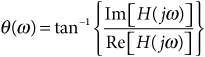
The steady-state frequency response of a linear system can be determined by evaluating the transfer function, H(s), at s = jω:

where θ(ω) is the phase response given by

and |H(jω)| is the magnitude response given by

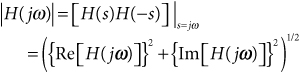
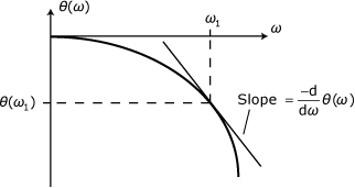
The group delay, τ_g(ω), is defined as

where θ(ω) is the phase response. As shown in Figure 39.1, the group delay at a frequency ω₁ is equal to the negative slope of a tangent to the phase response curve at the point corresponding to ω₁. Group delay is also called envelope delay because when a modulated carrier is passed through the system, the modulated envelope is delayed by τ_g. If the group delay is not consistent over the entire bandwidth of the signal, the envelope is distorted.

Figure 39.1. Group delay response

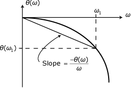
The phase delay, τ_p(ω), of a linear system is defined as

As depicted in Figure 39.2, the phase delay at a frequency ω₁ is equal to the negative slope of a secant drawn from the origin to the phase response curve at the point corresponding to ω₁. Phase delay is also called carrier delay because an unmodulated carrier at a frequency ω₁ experiences a delay of τ_p(ω) when passing through the system.

Figure 39.2. Phase delay response

39.3. Features of the Lowpass Response

The magnitude response for an analog lowpass filter will have one of the four general shapes shown in Figures 39.3 through 39.6. In each case, the filter response can be divided into three segments—the passband, the transition band, and the stopband. In some cases, the boundaries between these segments are defined by distinct features in the filter’s magnitude response, and sometimes the boundaries are based on an arbitrary line drawn on the magnitude response.

Figure 39.3. Monotonic magnitude response of a lowpass filter

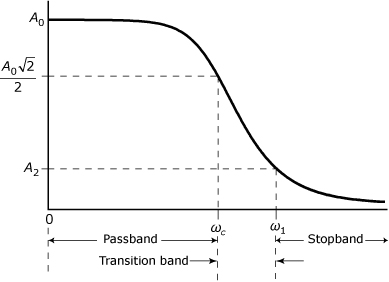
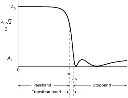
• The monotonic magnitude response shown in Figure 39.3 is an example of where the inter-band boundaries are defined by the frequencies at which the response crosses arbitrary levels. In most cases, the passband is defined to end when the magnitude response is 3 dB below the response level at zero frequency. Sometimes a different attenuation level such as 1 dB or 6 dB is used to define the end of the passband. In monotonic responses, there is almost no agreement regarding the level that sets the boundary between the transition band and the stopband. A Butterworth filter has a monotonic magnitude response.

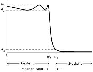
• The response shown in Figure 39.4 has ripples in the passband, and the troughs of the ripples define the level that defines the passband. The transition band begins when the response drops below the bottoms of the ripple troughs. If there is less than 3 dB of ripple in the passband, the 3 dB attenuation point is occasionally used to define the end of the passband. As with the monotonic response, there is no general agreement as to the level that should be used to define the beginning of the stopband. A Chebyshev filter has a response with ripples in the passband.

Figure 39.4. Magnitude response of a lowpass filter with ripples in the passband

• The response shown in Figure 39.5 has ripples in the stopband, and the crests of the ripple define the level that defines the stopband. The transition band ends and the stopband begins when the response first drops below the level corresponding to the ripple crests. The passband edge is defined as it is for the monotonic response. A Chebyshev Type 2 filter has a response with ripples in the stopband.

Figure 39.5. Magnitude response of a lowpass filter with ripples in the stopband

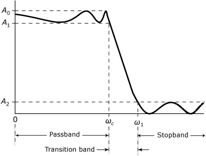
• The response shown in Figure 39.6 has ripples in both the passband and the stopband. The troughs in the passband ripple set the level that defines the end of the passband, and the crests in the stopband ripple set the level that defines the beginning of the stopband. An elliptic filter has a response with ripples in both the passband and the stopband.

Figure 39.6. Magnitude response of a lowpass filter with ripples in both the passband and the stopband.

39.4. Passband Transformations

When working with the classical filter families presented in Notes 40 through 43, it is common practice to first select a lowpass prototype filter having the appropriate characteristics and then transform this prototype into a bandpass or bandstop configuration as required. This note describes transformations that can be used to convert lowpass into bandpass or lowpass into bandstop. Similar transformations exist for converting lowpass into highpass, but highpass filters are rarely used in DSP applications.

Bandpass Transformation

Consider a lowpass filter normalized for 3-dB attenuation at frequency ω₀ and having a transfer function, H(S). There are a number of different transformations that can be used to map this proto type into a corresponding bandpass filter. The “conventional” transformation is based on evaluating H(S) at

39.1

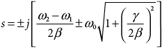
to obtain a filter with center frequency ω₀, lower 3-dB frequency ω₁, and upper 3-dB frequency ω₂. The properties of this transformation are examined in detail in [1]. If the lowpass prototype has zeros on the imaginary axis at S_i = ±jβ, each such pair transforms to two conjugate pairs of bandpass zeros on the imaginary axis:

39.2

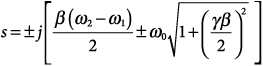
where γ is the relative bandwidth given by

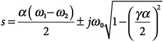
In order to use a lowpass protoype filter having a real-valued pole at S_i = –α, where α > 0, the frequencies of the bandpass filter must satisfy

39.3

If Eq. (39.3) is satisfied, the real lowpass pole transforms to the complex-conjugate pair of bandpass poles:

39.4

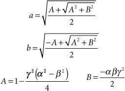
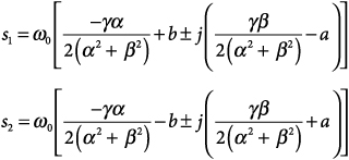
Each complex-conjugate pair of lowpass poles, –α ± jβ, transforms to two complex-conjugate pairs of bandpass poles given by

39.5

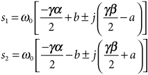
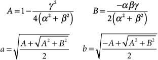
where

Bandstop Transformation

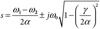
Consider a lowpass filter normalized for 3-dB attenuation at frequency ω₀ and having a transfer function, H(S). For mapping such a prototype into the corresponding bandstop filter, we can use a transformation that is based upon evaluating H(S) at

to obtain a bandstop filter with center frequency ω₀, lower 3-dB frequency ω₁, and upper 3-dB frequency ω₂. If the lowpass prototype has zeros on the imaginary axis at S_i = ±jβ, each such pair transforms to two conjugate pairs of bandstop zeros on the imaginary axis:

39.6

In order to use a lowpass prototype filter having a real-valued pole at S_i = –α, where α > 0, the frequencies of the bandpass filter must satisfy

39.7

If Eq. (39.7) is satisfied, this pole transforms to the complex-conjugate pair of bandstop poles:

39.8

Each complex-conjugate pair of lowpass poles –α ± jβ transforms to two complex-conjugate pairs of bandstop poles given by

where

References

1. H. J. Blinchikoff and A. I. Zverev, Filtering in the Time and Frequency Domains, Wiley-Interscience, New York, 1976.