
Note 46. Inverse z Transform via Partial Fraction Expansion:
Case 1: All Poles Distinct with M < N in System Function
This note covers the form of the partial fraction expansion that can be used to compute the inverse z transform of system functions that have no repeated poles and in which the degree of the denominator polynomial exceeds the degree of the numerator polynomial. The method is based on the basic strategy discussed in Note 45. Alternative approaches for use on system functions that do not meet these constraints are covered in Notes 47 through 49.
The form of the partial fraction expansion discussed in this note is suitable for use on system functions of the form
46.1
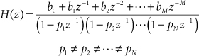
where M < N, thus making H(z) a proper rational function.
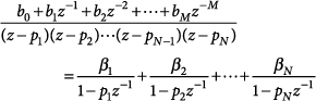
The expansion can be formed directly by using each binomial factor from the denominator of Eq. (46.1) as a denominator for one of the fractional terms in the expansion:
46.2
![]()
Design Procedure 46.1. Solving for PFE Coefficients: Coefficient Matching Approach
This procedure is appropriate for solving a partial fraction expansion of the form
DP 46.1
- Explicitly construct the RHS of Eq. (46.3) using the known values for the coefficients, bk, and poles, pk.
- Perform the necessary algebraic manipulations so that the coefficient for each power of z–1 on the right-hand side is obtained as a function of the unknown coefficients, βk
DP 46.2

- Set the coefficients from the LHS of Eq. (46.3) equal to the corresponding coefficients from the RHS of Eq. (DP 46.2):
DP 46.3
- Solve the system of linear equations (DP 46.3) for the coefficients βk.
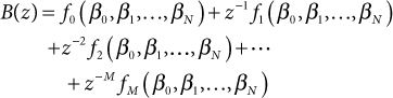
When a common denominator is generated to perform the additions indicated in Eq. (46.2), the resulting denominator always equals the denominator in Eq. (46.1). Therefore, we can simplify the notation by just retaining the numerator that results after the common denominator has been implemented to accomplish the additions. This “numerators-only” equation has the form
46.3

Typically, the values for all the poles, pk, are known, so straightforward algebraic manipulations can be used to put the right-hand side of Eq. (46.3) into a form in which the coefficient for each power of z–1 is obtained as a function of the unknown coefficients, βnk:
46.4
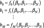
Coefficients for like powers of z must have the same value in the LHS of Eq. (46.3) and in the RHS of Eq. (46.4) so we can construct the system of equations
46.5

From the form of the RHS of Eq. (46.3), we know that each function, fm(β0, β1, . . ., βN), is a linear function of the coefficients, βn, so it is a straightforward process to solve this system of equations for the unknown values of βn.
Once the values for the βn are found, the filter’s unit sample response can be written as
46.6
![]()
This approach for computing the inverse z transform is summarized in Design Procedure 46.1, and is demonstrated in Example 46.1.
Example 46.1. Coefficient Matching Approach When H(z) Is a Proper Rational Function
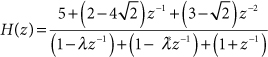
Consider the system function given by
46.7

The denominator can be factored to yield
46.8
where
46.9
![]()
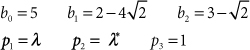
In terms of the notation used in Design Procedure 46.1, we have
46.10
Expanding Eq. (46.8) in the form of Eq. (46.2) yields
46.11
![]()
Finding a common denominator to add the right-hand side yields a numerator of
46.12

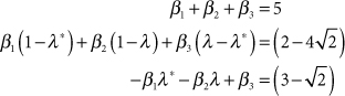
Setting the coefficients from Eq. (46.12) equal to the numerator coefficients from Eq. (46.8) for like powers of z yields the system of equations
46.13
Substituting the values for λ and λ, and then solving for β1, β2, and β3 yields
46.14
![]()
Thus, the unit sample response is given by
46.15
![]()