
Note 6. Natural Sampling
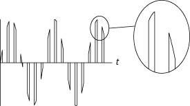
In natural sampling, an analog signal is gated in such a way that the resulting signal consists of pulses with time-varying amplitudes that follow the contours of the original waveform as shown in Figure 6.1. In this example, the original signal is a sinusoid with a period of Tx, and the sampled signal has a sampling interval of T, and a sample width of τ. Natural sampling is mathematically equivalent to multiplying the original signal with a train of unit-amplitude rectangular sampling pulses. Therefore, the spectrum of a naturally sampled signal can be determined by convolving the original signal’s spectrum with the spectrum of the train of sampling pulses.
Figure 6.1. In natural samping, the amplitudes of the sample pulses follow the varying amplitudes of the original function.
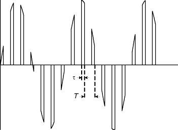
Figure 6.2 summarizes the relationships between the original signal (labeled T4), the naturally sampled signal (labeled T5), and the corresponding spectra (labeled F4 and F5, respectively). The train of sampling pulses (labeled T3) can be generated by convolving a single pulse of width τ (labeled T1) with a Dirac comb having impulses spaced at intervals of T (labeled T2). The resulting pulse train has a magnitude spectrum like the one shown in Figure 6.3.
Figure 6.2. Natural sampling is mathematically equivalent to multiplying the original spectrum with a train of rectangular sampling pulses. Therefore, the spectrum of a naturally sampled signal can be determined by convolving the original signal’s spectrum with the spectrum of the train of sampling pulses. (The multiply operation that creates spectrum F3 is not mathematically rigorous, but it is consistent with typical engineering use of Dirac delta functions as discussed in Note 5. “CTFT” indicates the continuous-time Fourier transform.)
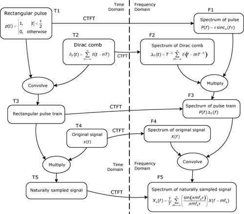
Figure 6.3. Magnitude spectrum of rectangular pulse train (corresponds to block F3 in Figure 6.2)
At a Glance
• Natural sampling is a mathematical model that can be used to analyze the impacts of analog multiplexing and signal commutation and decommutation.
• In natural sampling, the samples have nonzero width and the amplitude of the sample varies across the width of the sample to match the amplitude of the analog signal.
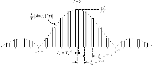
• In the magnitude spectrum of a naturally sampled signal, each image is scaled by a factor that is constant over the image but that varies from image to image according to the magnitude of a sinc envelope.

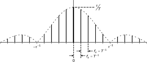
The magnitude spectrum for a naturally sampled sinusoid is shown in Figure 6.4. The spacing of the images is equal to the reciprocal of the sampling interval, and each image is amplitude scaled by the value of τT–1|sincπ(fτ)| at the frequency corresponding to the center of the image. In other words, the image centered at f = nfs is scaled by τT–1|sincπ(nfsτ)|. This factor changes from image to image, but remains constant across the width of each image.
Figure 6.4. Magnitude spectrum of naturally sampled sinusoid (corresponds to block F5 in Figure 6.2)
Reference
1. W. R. Bennett, “Time division multiplex systems,” Bell Syst. Tech. J., vol. 20, 1941, pp. 199–221.