Note 23. Window Characteristics
There are many different window functions, and selecting the best one for a particular application can be a daunting task. However there are a number of metrics that can be used to weed out the unsuitable windows and zero in on the several “best” window choices for particular requirements.
23.1. Main Lobe Width
Any window having a finite duration in time has a frequency-domain magnitude response that exhibits a lobed structure similar to the example shown in Figure 23.1. Perhaps the most obvious quantifiable characteristic for a window concerns the width of the main lobe in the magnitude response. The null-to-null measurement is a conceptually straightforward way to characterize the width of the main lobe, but it is not the most useful way.
Figure 23.1. DTFT response of a rectangular window showing the features of the response’s lobed structure
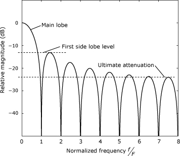
The 6-dB bandwidth of the main lobe is a useful metric because for two equal-strength tones to be resolvable in the output of a windowed DTFT, their frequencies must differ by more than the 6-dB bandwidth of the window.
The 3-dB bandwidth of the main lobe is also useful because it can be combined with the equivalent noise bandwidth, discussed later, in section 23.3, to form an indicator of window performance. Specifically, in [1], harris compared more than 40 different windows, and based on DFT results for these windows, he concluded that the ratio of equivalent noise bandwidth to 3-dB bandwidth is a sensitive indicator of overall window performance. Of the windows he tested, good windows always had bandwidth ratios that satisfied
23.1
![]()
Windows with this ratio less than 1.04 had wide main lobes that resulted in high processing loss. Windows with this ratio greater than 1.055 tended to have high side lobe structure that resulted in poor two-tone detection capability.
23.2. Side Lobe Attenuation
There are two useful measures of side lobe attenuation.
- Peak level of the first side lobe.
- Ultimate attenuation of side lobes far removed from the main lobe. In the case of discrete-time windows, the ultimate attenuation is the attenuation at the side lobe peak closest to ω = π.
Poor side lobe attenuation degrades the two-tone detection capability of a window, especially in cases where one tone is much stronger than the other. Even when the tones’ frequencies are separated by more than the 6-dB bandwidth of the window’s main lobe, the weaker signal often is lost in the side lobes of the stronger signal’s response.
Poor side lobe attenuation also causes bias in the amplitude and frequency estimates formed by the DFT. The side lobes of the negative-frequency component for a tone create bias in the positive-frequency component, and the side lobes of the positive-frequency component create bias in the negative-frequency component.
23.3. Equivalent Noise Bandwidth
The magnitude-squared response for a typical window function is shown in Figure 23.2. If the window function is applied to a signal consisting of zero-mean white noise, the total noise power in the result can be computed in the frequency domain as
23.2
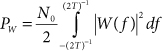
Figure 23.2. Equivalent noise bandwidth. The total area under the curve equals the area of the dashed rectangle.
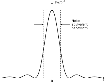
Figure 23.2 also shows a dashed-line rectangle that can be thought of as the magnitude response of an ideal lowpass filter. This rectangle has a height equal to the peak in the window’s response and a width equal to 2Bneq. The output noise power from the ideal filter is
23.3
![]()
The value of B for which the window and the ideal filter produce the same output noise power is called the equivalent noise bandwidth1, and is found by equating Eqs. (23.2) and (23.3) and solving for B to yield
23.4
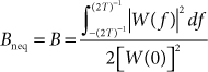
We can invoke Parseval’s theorem to obtain time-domain expressions for the numerator and denominator of Eq. (23.4) to yield a more convenient equation for Bneq that is based directly on the time-domain window function
23.5
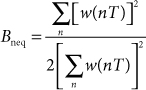
The index limits for the summations are not stated explicitly, because in some applications n will range from –N/2 through N/2 and in other applications n will range from 0 through N –1.
23.4. Processing Gain
The processing gain of a windowed transform can be analyzed by considering the DFT to be a bank of matched filters, with each filter matched to a sinusoid at one of the bin frequencies, ωk. The windowed transform’s processing gain, GP, is defined as the ratio of output signal-to-noise ratio (SNR) to input SNR, when the input to the transform is a noisy sinusoid at one of the transform’s bin frequencies:
23.6
![]()
when the input signal is defined by
23.7
![]()
where
23.8
![]()
and ρ(nT) is a white noise sequence with variance ![]() . The input signal power is simply Sin = A2, and the input noise power is
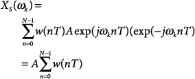
. The input signal power is simply Sin = A2, and the input noise power is ![]() . That portion of the windowed transform’s output that is due to signal is given by
. That portion of the windowed transform’s output that is due to signal is given by
23.9
and the corresponding signal power is given by
23.10
![]()
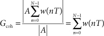
The coherent gain is defined as the magnitude of the output signal divided by the magnitude of the input signal:
23.11
The portion of the windowed transform’s output due to noise is given by
23.12
![]()
and the output noise power is the mean-square value of XN (ωk):
23.13
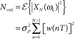
Thus, the processing gain can be determined as
23.14
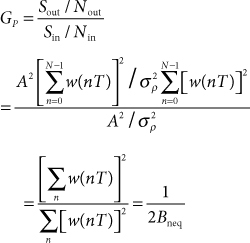
where Bneq is the equivalent noise bandwidth discussed in Section 23.3. The processing loss, LP, is the reciprocal of the processing gain
23.15
![]()
23.5. Scalloping Loss
The processing loss computed in the previous section is based on an input signal that is a sinusoid at a frequency corresponding to one of the DFT bin frequencies. There will be additional loss for an input sinusoid at any frequency that is not one of the bin frequencies. The maximum loss will occur for an input frequency that is exactly midway between two consecutive bin frequencies. The input signal becomes
x[n] = A exp(jω(k + 1/2)nT) + ρ (nT)
where
![]()
The portion of the windowed transform’s output in bin k that is due to a noise-free sinusoidal signal of frequency ω(k+1/2) is then given by
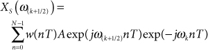
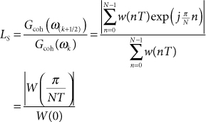
After some trigonometric manipulation, this output component can be expressed as
![]()
The scalloping loss is defined as the ratio of the coherent gain for a signal midway between two bin frequencies to the coherent gain for a signal at a bin frequency:
23.16
23.6. Worst Case Processing Loss
The worst case processing loss is defined as the product of the processing loss from Eq. (23.15) and the scalloping loss from Eq. (23.16).
References
1. f. j. harris, “On the Use of Windows for Harmonic Analysis with the Discrete Fourier Transform,” Proc. IEEE, vol. 66, no. 1, January 1978, pp. 51–83.