
10.2 Memory Management
Let’s review what we said about main memory in Chapter 5. All programs are stored in main memory when they are executed. All data referenced by those programs are also stored in main memory so that they can be accessed. Main memory can be thought of as a big, continuous chunk of space divided into groups of 8, 16, or 32 bits. Each byte or word of memory has a corresponding address, which is simply an integer that uniquely identifies that particular part of memory. See FIGURE 10.4. The first memory address is 0.

FIGURE 10.4 Memory is a continuous set of bits referenced by specific addresses
Earlier in this chapter we stated that in a multiprogramming environment, multiple programs (and their data) are stored in main memory at the same time. Thus operating systems must employ techniques to perform the following tasks:
■ Track where and how a program resides in memory
■ Convert logical program addresses into actual memory addresses
A program is filled with references to variables and to other parts of the program code. When the program is compiled, these references are changed into the addresses in memory where the data and code reside. But given that we don’t know exactly where a program will be loaded into main memory, how can we know which address to use for anything?
The solution is to use two kinds of addresses: logical addresses and physical addresses. A logical address (sometimes called a virtual or relative address) is a value that specifies a generic location relative to the program but not to the reality of main memory. A physical address is an actual address in the main memory device, as shown in Figure 10.4.
When a program is compiled, a reference to an identifier (such as a variable name) is changed to a logical address. When the program is eventually loaded into memory, each logical address is translated into a specific physical address. The mapping of a logical address to a physical address is called address binding. The later we wait to bind a logical address to a physical one, the more flexibility we have. Logical addresses allow a program to be moved around in memory or loaded in different places at different times. As long as we keep track of where the program is stored, we can always determine the physical address that corresponds to any given logical address. To simplify our examples in this chapter, we perform address-binding calculations in base 10.
The following sections examine the underlying principles of three techniques:
■ Single contiguous memory management
■ Partition memory management
■ Paged memory management
Single Contiguous Memory Management
Let’s initially keep things simple by assuming that there are only two programs in memory: the operating system and the application program we want to execute. We divide main memory up into two sections, one for each program, as shown in FIGURE 10.5. The operating system gets what space it needs, and the program is allocated the rest.

FIGURE 10.5 Main memory divided into two sections
This approach is called single contiguous memory management because the entire application program is loaded into one large chunk of memory. Only one program other than the operating system can be processed at one time. To bind addresses, all we have to take into account is the location of the operating system.
In this memory management scheme, a logical address is simply an integer value relative to the starting point of the program. That is, logical addresses are created as if the program loaded at location 0 of main memory. Therefore, to produce a physical address, we add a logical address to the starting address of the program in physical main memory.
Let’s get a little more specific: If the program is loaded starting at address A, then the physical address corresponding to logical address L is A + L. See FIGURE 10.6. Let’s plug in real numbers to make this example clearer. Suppose the program is loaded into memory beginning at address 555555. When a program uses relative address 222222, we know that it is actually referring to address 777777 in physical main memory.
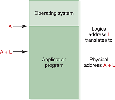
FIGURE 10.6 Binding a logical address to a physical address
It doesn’t really matter what address L is. As long as we keep track of A (the starting address of the program), we can always translate a logical address into a physical one.
You may be saying at this point, “If we switched the locations of the operating system and the program, then the logical and physical addresses for the program would be the same.” That’s true. But then you’d have other things to worry about. For example, a memory management scheme must always take security into account. In particular, in a multiprogramming environment, we must prevent a program from accessing any addresses beyond its allocated memory space. With the operating system loaded at location 0, all logical addresses for the program are valid unless they exceed the bounds of main memory itself. If we move the operating system below the program, we must make sure a logical address doesn’t try to access the memory space devoted to the operating system. This wouldn’t be difficult, but it would add to the complexity of the processing.
The advantage of the single contiguous memory management approach is that it is simple to implement and manage. However, it almost certainly wastes both memory space and CPU time. An application program is unlikely to need all of the memory not used by the operating system, and CPU time is wasted when the program has to wait for some resource.
Partition Memory Management
Once multiple programs are allowed in memory, it’s the operating system’s job to ensure that one program doesn’t access another’s memory space. This is an example of a security mechanism implemented at a low level, generally outside the knowledge of the user. Higher-level issues are discussed in Chapter 17.
A more sophisticated approach is to have more than one application program in memory at the same time, sharing memory space and CPU time. In this case, memory must be divided into more than two partitions. Two strategies can be used to partition memory: fixed partitions and dynamic partitions. With the fixed-partition technique, main memory is divided into a particular number of partitions. The partitions do not have to be the same size, but their size is fixed when the operating system initially boots. A job is loaded into a partition large enough to hold it. The OS keeps a table of addresses at which each partition begins and the length of the partition.
With the dynamic-partition technique, the partitions are created to fit the unique needs of the programs. Main memory is initially viewed as one large empty partition. As programs are loaded, space is “carved out,” using only the space needed to accommodate the program and leaving a new, smaller, empty partition, which may be used by another program later. The operating system maintains a table of partition information, but in dynamic partitions the address information changes as programs come and go.
At any point in time in both fixed and dynamic partitions, memory is divided into a set of partitions, some empty and some allocated to programs. See FIGURE 10.7.
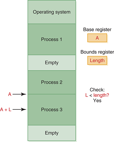
FIGURE 10.7 Address resolution in partition memory management
Address binding is basically the same for both fixed and dynamic partitions. As with the single contiguous memory management approach, a logical address is an integer relative to a starting point of 0. There are various ways an OS might handle the details of the address translation. One way is to use two special-purpose registers in the CPU to help manage addressing. When a program becomes active on the CPU, the OS stores the address of the beginning of that program’s partition into the base register. Similarly, the length of the partition is stored in the bounds register. When a logical address is referenced, it is first compared to the value in the bounds register to make sure the reference is within that program’s allocated memory space. If it is, the value of the logical address is added to the value in the base register to produce the physical address.
Which partition should we allocate to a new program? There are three general approaches to partition selection:
■ First fit, in which the program is allocated to the first partition big enough to hold it
■ Best fit, in which the program is allocated to the smallest partition big enough to hold it
■ Worst fit, in which the program is allocated to the largest partition big enough to hold it
It doesn’t make sense to use worst fit in fixed partitions because it would waste the larger partitions. First fit and best fit both work for fixed partitions. In dynamic partitions, however, worst fit often works best because it leaves the largest possible empty partition, which may accommodate another program later on.
When a program terminates, the partition table is updated to reflect the fact that the partition is now empty and available for a new program. In dynamic partitions, consecutive empty partitions are merged into one big empty partition.
Partition memory management makes efficient use of main memory by maintaining several programs in memory at one time. But keep in mind that a program must fit entirely into one partition. Fixed partitions are easier to manage than dynamic ones, but they restrict the opportunities available to incoming programs. The system may have enough free memory to accommodate the program, just not in one free partition. In dynamic partitions, the jobs could be shuffled around in memory to create one large free partition. This procedure is known as compaction.
Paged Memory Management
Paged memory management places more of the burden on the operating system to keep track of allocated memory and to resolve addresses. However, the benefits gained by this approach are generally worth the extra effort.
In the paged memory technique, main memory is divided into small fixed-size blocks of storage called frames. A process is divided into pages that (for the sake of our discussion) we assume are the same size as a frame. When a program is to be executed, the pages of the process are loaded into unused frames distributed through memory. Thus the pages of a process may be scattered around, out of order, and mixed among the pages of other processes. To keep track of these pages, the operating system maintains a separate page-map table (PMT) for each process in memory; it maps each page to the frame in which it is loaded. See FIGURE 10.8 Both pages and frames are numbered starting with zero, which makes the address calculations easier.
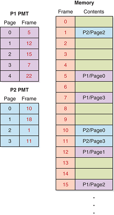
FIGURE 10.8 A paged memory management approach
A logical address in a paged memory management system begins as a single integer value relative to the starting point of the program, as it was in a partitioned system. This address is modified into two values, a page number and an offset, by dividing the address by the page size. The page number is the number of times the page size divides the address, and the remainder is the offset. So a logical address of 2566, with a page size of 1024, corresponds to the 518th byte of page 2 of the process. A logical address is often written as <page, offset>, such as <2, 518>.
To produce a physical address, you first look up the page in the PMT to find the frame number in which it is stored. You then multiply the frame number by the frame size and add the offset to get the physical address. For example, given the situation shown in FIGURE 10.8 , if process 1 is active, a logical address of <1, 222> would be processed as follows: Page 1 of process 1 is in frame 12; therefore, the corresponding physical address is 12 * 1024 + 222, or 12510. Note that there are two ways in which a logical address could be invalid: The page number could be out of bounds for that process, or the offset could be larger than the size of a frame.
The advantage of paging is that a process no longer needs to be stored contiguously in memory. The ability to divide a process into pieces changes the challenge of loading a process from finding one large chunk of space to finding many small chunks.
An important extension to the idea of paged memory management is the idea of demand paging, which takes advantage of the fact that not all parts of a program actually have to be in memory at the same time. At any given point in time, the CPU is accessing one page of a process. At that point, it doesn’t really matter whether the other pages of that process are even in memory.
In demand paging, the pages are brought into memory on demand. That is, when a page is referenced, we first see whether it is in memory already and, if it is, complete the access. If it is not already in memory, the page is brought in from secondary memory into an available frame, and then the access is completed. The act of bringing in a page from secondary memory, which often causes another page to be written back to secondary memory, is called a page swap.
The demand paging approach gives rise to the idea of virtual memory, the illusion that there are no restrictions on the size of a program (because the entire program is not necessarily in memory at the same time). In all of the memory management techniques we examined earlier, the entire process had to be brought into memory as a continuous whole. We therefore always had an upper bound on process size. Demand paging removes that restriction.
However, virtual memory comes with lots of overhead during the execution of a program. With other memory management techniques, once a program was loaded into memory, it was all there and ready to go. With the virtual memory approach, we constantly have to swap pages between main and secondary memory. This overhead is usually acceptable— while one program is waiting for a page to be swapped, another process can take control of the CPU and make progress. Excessive page swapping is called thrashing and can seriously degrade system performance.