
7.4 Searching Algorithms
The act of searching is a common activity for humans as well as computers. When you look for a name in a directory, for instance, you are performing a search. We explore two search algorithms in this section.
Sequential Search
Our first searching algorithm follows the most straightforward concept of a search. We look at each item in turn and compare it to the one for which we are searching. If it matches, we have found the item. If not, we look at the next item. We stop either when we have found the item or when we have looked at all the items and not found a match. This sounds like a loop with two ending conditions. Let’s write the algorithm using the array numbers.
Because we have a compound condition in the WHILE expression, we need to say a little more about Boolean variables. AND is a Boolean operator. The Boolean operators include the special operators AND, OR, and NOT. The AND operator returns TRUE if both expressions are TRUE, and FALSE otherwise. The OR operator returns FALSE if both expressions are FALSE, and TRUE otherwise. The NOT operator changes the value of the expression. These operations are consistent with the functionality of the gates described in Chapter 4. At that level, we were referring to the flow of electricity and the representation of individual bits. At this level, the logic is the same, but we can talk in terms of an expression as being either true or false.
We can simplify the second Boolean expression (found is FALSE) by using the NOT operator. NOT found is true when found is false. So we can say
WHILE (position < 10 AND NOT found)
Thus, the loop will repeat as long as the index is less than 10 and we haven’t found the matching item.
Sequential Search in a Sorted Array
If we know that the items in the array are sorted, we can stop looking when we pass the place where the item would be if it were present in the array. As we look at this algorithm, let’s generalize our search somewhat. Rather than being specific about the number of items in the array, we use a variable length to tell us how many valid items are in the array. The length might be less than the size, which is the number of slots in the array. As data is being read into the array, a counter is updated so that we always know how many data items were stored. If the array is called data, the data with which we are working is from data[0] to data[length – 1]. FIGURES 7.7 and 7.8 show an unordered array and a sorted array, respectively.
![A figure of the unsorted array named list of length 6 reads from the index [0] to [max_length -1 ] from top to bottom: 60, 75, 95, 80, 65, and 90. The portion between index [5] to [max_length -1 ] is left empty.](http://images-20200215.ebookreading.net/5/1/1/9781284155648/9781284155648__computer-science-illuminated__9781284155648__images__9781284156010_CH07_FIG07.png)
FIGURE 7.7 An unsorted array
![A figure of the sorted array named list of length 6 reads from the index [0] to [max_length -1 ] from top to bottom as 60, 65, 75, 80, 90, and 95. The portion between index [5] to [max_length -1 ] is left empty.](http://images-20200215.ebookreading.net/5/1/1/9781284155648/9781284155648__computer-science-illuminated__9781284155648__images__9781284156010_CH07_FIG08.png)
FIGURE 7.8 A sorted array
In the sorted array, if we are looking for 76, we know it is not in the array as soon as we examine data[3], because this position is where the number would be if it were there. Here is the algorithm for searching in a sorted array embedded in a complete program. We use the variable index rather than position in this algorithm. Programmers often use the mathematical identifier index rather than the intuitive identifier position or place when working with arrays.
Binary Search
How would you go about looking for a word in a dictionary? We certainly hope you wouldn’t start on the first page and sequentially search for your word! A sequential search of an array begins at the beginning of the array and continues until the item is found or the entire array has been searched without finding the item.
A binary search looks for an item in an array using a different strategy: divide and conquer. This approach mimics what you probably do when you look up a word. You start in the middle and then decide whether your word is in the right-hand section or the left-hand section. You then look in the correct section and repeat the strategy.
The binary search algorithm assumes that the items in the array being searched are sorted, and it either finds the item or eliminates half of the array with one comparison. Rather than looking for the item starting at the beginning of the array and moving forward sequentially, the algorithm begins at the middle of the array in a binary search. If the item for which we are searching is less than the item in the middle, we know that the item won’t be in the second half of the array. We then continue by searching the data in the first half of the array. See FIGURE 7.9.
![A figure of the binary search array named ‘Items’ of length 11 from the index [0] to [10] (and goes) reads from top to bottom: ant, cat, chicken, cow, deer, dog, fish, goat, horse, rat, and snake. The remaining portion is left empty.](http://images-20200215.ebookreading.net/5/1/1/9781284155648/9781284155648__computer-science-illuminated__9781284155648__images__9781284156010_CH07_FIG09.png)
FIGURE 7.9 Binary search example
Once again we examine the “middle” element (which is really the item 25% of the way into the array). If the item for which we are searching is greater than the item in the middle, we continue searching between the middle and the end of the array. If the middle item is equal to the one for which you are searching, the search stops. The process continues in this manner, with each comparison cutting in half the portion of the array where the item might be. It stops when the item is found or when the portion of the array where the item might be is empty.
Let’s desk check (walk through) the algorithm, searching for cat, fish, and zebra. Rather than boxes, we use a tabular form in FIGURE 7.10 to save space.
Is the binary search algorithm really faster than the sequential search algorithm? TABLE 7.1 shows the number of comparisons required on average to find an item using a sequential search and using a binary search. If the binary search is so much faster, why don’t we always use it? More computations are required for each comparison in a binary search because we must calculate the middle index.
| TABLE | ||
| 7.1 Average Number of Comparisons | ||
| Length | Sequential Search | Binary Search |
| 10 | 5.5 | 2.9 |
| 100 | 50.5 | 5.8 |
| 1000 | 500.5 | 9.0 |
| 10000 | 5000.5 | 12.0 |
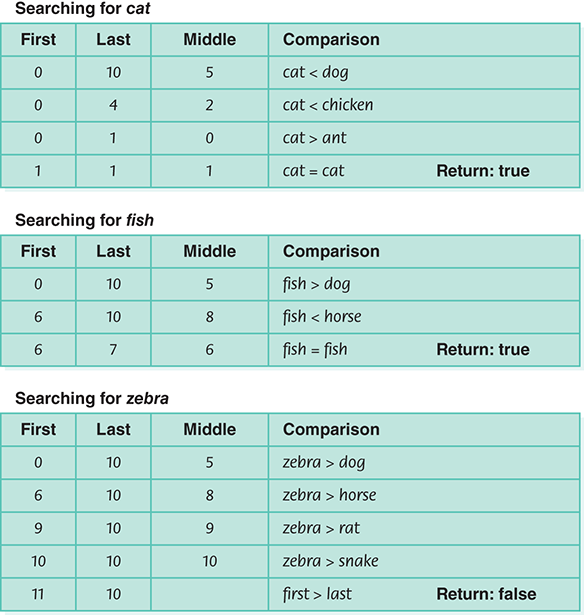
FIGURE 7.10 Trace of the binary search
Also, the array must already be sorted. If the array is already sorted and the number of items is more than 20, a binary search algorithm is the better choice.