
8.6 Graphs
Trees are a useful way to represent relationships in which a hierarchy exists. That is, a node is pointed to by at most one other node (its parent). If we remove the restriction that each node may have only one parent node, we have a data structure called a graph. A graph is made up of a set of nodes called vertices and a set of lines called edges (or arcs) that connect the nodes.
The vertices in the graph represent objects, and the edges describe relationships among the vertices. For instance, if the graph is representing a map, the vertices might be the names of cities, and the edges that link the vertices could represent roads between pairs of cities. Because the roads that run between cities are two-way paths, the edges in this graph have no direction. Such a graph is called an undirected graph. However, if the edges that link the vertices represent flights from one city to another, the direction of each edge is important. The existence of a flight (edge) from Houston to Austin does not assure the existence of a flight from Austin to Houston. A graph whose edges are directed from one vertex to another is called a directed graph (or digraph). A weighted graph is one in which there are values attached to the edges in the graph.
Look at the graphs in FIGURE 8.10. The relationships among siblings are undirected. For example, June is Sarah’s sibling and Sarah is June’s sibling; see FIGURE 8.10(a). The prerequisite chart in FIGURE 8.10(c) is directed: Computer Science I must come before Computer Science II. The flight schedule is both directed and weighted; see FIGURE 8.10(b). There is a flight from Dallas to Denver that covers a distance of 780 miles, but there is not a direct flight from Denver to Dallas.
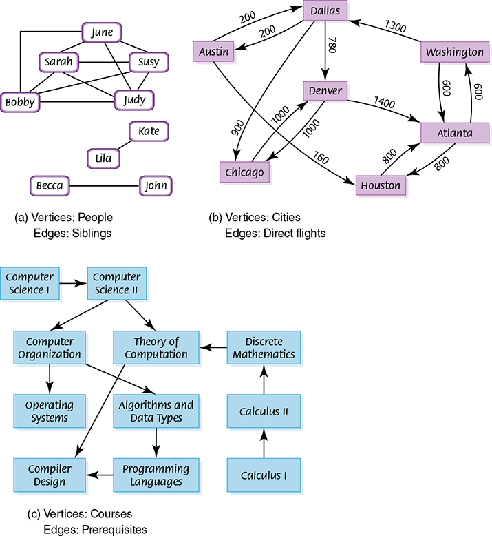
FIGURE 8.10 Examples of graphs
If two vertices are connected by an edge, we say they are adjacent vertices. In Figure 8.10(a), June is adjacent to Bobby, Sarah, Judy, and Susy. A path from one vertex to another consists of a sequence of vertices that connect them. For example, there is a path from Austin to Dallas to Denver to Chicago. There is not a path from June to Lila, Kate, Becca, or John.
Vertices represent whatever objects are being modeled: people, houses, cities, courses, concepts, and so on. The edges represent relationships between those objects. For example, people are related to other people, houses are on the same street, cities are linked by direct flights, courses have prerequisites, and concepts are derived from other concepts. (See Figure 8.10.) Mathematically, vertices are the undefined concept upon which graph theory rests. There is a great deal of formal mathematics associated with graphs, which is beyond the scope of this book.
Creating a Graph
Lists, stacks, queues, and trees are all just holding containers. The user chooses which is most appropriate for a particular problem. There are no inherent semantics other than those built into the retrieval process: A stack returns the item that has been in the stack the least amount of time; a queue returns the item that has been in the queue the longest amount of time. Lists and trees return the information that is requested. A graph, in contrast, has algorithms defined upon it that actually solve classic problems. First we talk about building a graph; then we discuss problems that are solvable using a graph.
A lot of information is represented in a graph: the vertices, the edges, and the weights. Let’s visualize the structure as a table using the flight connection data. The rows and columns in TABLE 8.3 are labeled with the city names. A zero in a cell indicates that there is no flight from the row city to the column city. The values in the table represent the number of miles from the row city to the column city.
| TABLE | ||
| 8.3 Data for the Flight Graph | ||

|
||
To build such a table we must have the following operations:
Add a vertex to the table
Add an edge to the table
Add a weight to the table
We find a position in the table by stating the row name and the column name. That is, (Atlanta, Houston) has a flight of 800 miles. (Houston, Austin) contains a zero, so there is no direct flight from Houston to Austin.
Graph Algorithms
There are three classic searching algorithms defined on a graph, each of which answers a different question.
Can I get from City X to City Y on my favorite airline?
How can I fly from City X to City Y with the fewest number of stops?
What is the shortest flight (in miles) from City X to City Y?
The answers to these three questions involve a depth-first search, a breadth-first search, and a single-source shortest-path search.
Depth-First Search
Can I get from City X to City Y on my favorite airline? Given a starting vertex and an ending vertex, let’s develop an algorithm that finds a path from startVertex to endVertex. We need a systematic way to keep track of the cities as we investigate them. Let’s use a stack to store vertices as we encounter them in trying to find a path between the two vertices. With a depth-first search, we examine the first vertex that is adjacent with startVertex; if this is endVertex, the search is over. Otherwise, we examine all the vertices that can be reached in one step from this first vertex.
Meanwhile, we need to store the other vertices that are adjacent with startVertex to use later if we need them. If a path does not exist from the first vertex adjacent with startVertex, we come back and try the second vertex, third vertex, and so on. Because we want to travel as far as we can down one path, backtracking if endVertex is not found, a stack is the appropriate structure for storing the vertices.
We mark a vertex as visited once we have put all its adjacent vertices on the stack. If we process a vertex that has already been visited, we keep putting the same vertices on the stack over and over again. Then the algorithm isn’t an algorithm at all because it might never end. So we must not process a vertex more than once.
Let’s apply this algorithm to the sample airline-route graph in Figure 8.10(b). We want to fly from Austin to Washington. We initialize our search by pushing our starting city onto the stack (FIGURE 8.11(a)). At the beginning of the loop, we pop the current city, Austin, from the stack. The places we can reach directly from Austin are Dallas and Houston; we push both these vertices onto the stack (FIGURE 8.11(b)). At the beginning of the second iteration, we pop the top vertex from the stack—Houston. Houston is not our destination, so we resume our search from there. There is only one flight out of Houston, to Atlanta; we push Atlanta onto the stack (FIGURE 8.11(c)). Again we pop the top vertex from the stack. Atlanta is not our destination, so we continue searching from there. Atlanta has flights to two cities: Houston and Washington.
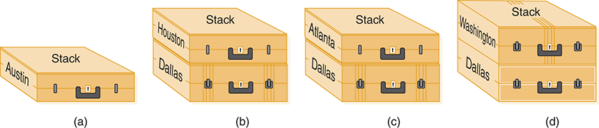
FIGURE 8.11 Using a stack to store the routes
But we just came from Houston! We don’t want to fly back to cities that we have already visited; this could cause an infinite loop. But we have already taken care of this problem: Houston has already been visited, so we continue without putting anything on the stack. The second adjacent vertex, Washington, has not been visited, so we push it onto the stack (FIGURE 8.11(d)). Again we pop the top vertex from the stack. Washington is our destination, so the search is complete.
FIGURE 8.12 shows the result of asking if we can reach Washington from Austin.
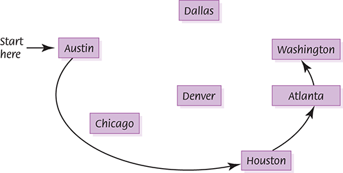
FIGURE 8.12 The depth-first search
This search is called a depth-first search because we go to the deepest branch, examining all the paths beginning at Houston before we come back to search from Dallas. When you have to backtrack, you take the branch closest to where you dead-ended. That is, you go as far as you can down one path before you take alternative choices at earlier branches.
Breadth-First Search
How can you get from City X to City Y with the fewest number of stops? The breadth-first traversal answers this question. When we come to a dead end in a depth-first search, we back up as little as possible. We try another route from the most recent vertex—the route on top of our stack. In a breadth-first search, we want to back up as far as possible to find a route originating from the earliest vertices. The stack is not the right structure for finding an early route. It keeps track of things in the order opposite of their occurrence—that is, the latest route is on top. To keep track of things in the order in which they happen, we use a queue. The route at the front of the queue is a route from an earlier vertex; the route at the back of the queue is from a later vertex. Thus, if we substitute a queue for a stack, we get the answer to our question.
Let’s apply this algorithm to the same airline-route graph in Figure 8.10(b). Which path gives us the route from Austin to Washington with the fewest stops? Austin is in the queue to start the process (FIGURE 8.13(a) ). We dequeue Austin and enqueue all the cities that can be reached directly from Austin: Dallas and Houston (FIGURE 8.13(b) ). Then we dequeue the front queue element. Dallas is not the destination we seek, so we enqueue all the adjacent cities that have not yet been visited: Chicago and Denver (FIGURE 8.13(c) ). (Austin has been visited already, so it is not enqueued.) Again we dequeue the front element from the queue. This element is the other “one-stop” city—Houston. Houston is not the desired destination, so we continue the search. There is only one flight out of Houston, and it is to Atlanta. Because we haven’t visited Atlanta before, it is enqueued (FIGURE 8.13(d) ).
Now we know that we cannot reach Washington with one stop, so we start examining the two-stop connections. We dequeue Chicago; this is not our destination, so we put its adjacent city, Denver, into the queue (FIGURE 8.13(e) ). Now this is an interesting situation: Denver is in the queue twice. We have put Denver into the queue in one step and removed its previous entry at the next step. Denver is not our destination, so we put its adjacent cities that haven’t been visited (only Atlanta) into the queue (FIGURE 8.13(f) ).This processing continues until Washington is put into the queue (from Atlanta) and is finally dequeued. We have found the desired city, and the search is complete (FIGURE 8.14 ).
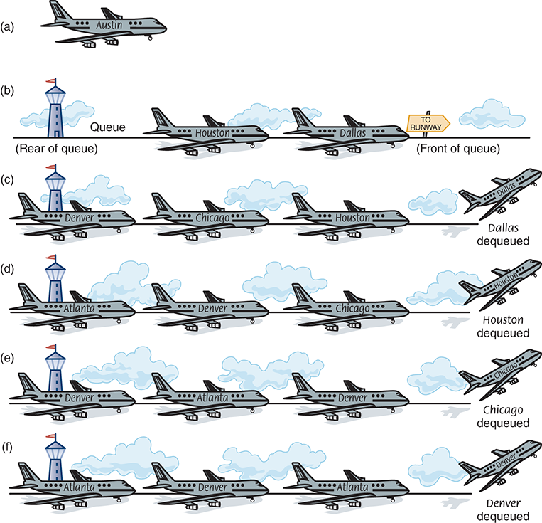
FIGURE 8.13 Using a queue to store the routes
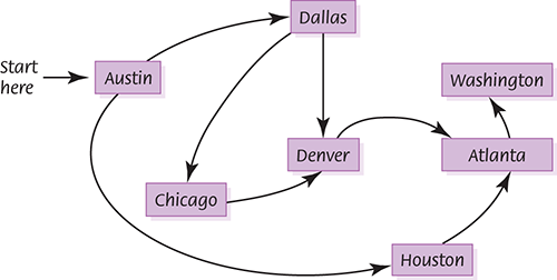
FIGURE 8.14 The breadth-first search
As you can see from these two algorithms, a depth-first search goes as far down a path from startVertex as it can before looking for a path beginning at the second vertex adjacent with startVertex. In contrast, a breadth-first search examines all of the vertices adjacent with startVertex before looking at those adjacent with these vertices.
Single-Source Shortest-Path Search
What is the shortest flight (in miles) from Austin to some other city? We know from the two search operations just discussed that there may be multiple paths from one vertex to another. Suppose we want to find the shortest path from Austin to each of the other cities that your favorite airline serves. By “shortest path,” we mean the path whose edge values (weights), when added together, have the smallest sum. Consider the following two paths from Austin to Washington:

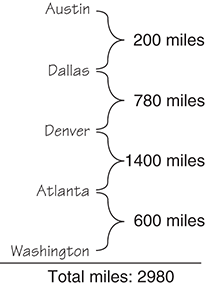
Clearly the first path is preferable, unless you want to collect frequent-flyer miles.
Let’s develop an algorithm that displays the shortest path from a designated starting city to every other city in the graph—this time we are not searching for a path between a starting city and an ending city. As in the two graph searches described earlier, we need an auxiliary structure for storing cities that we process later. By retrieving the city that was most recently put into the structure, the depth-first search tries to keep going “forward.” It tries a one-flight solution, then a two-flight solution, then a three-flight solution, and so on. It backtracks to a fewer-flight solution only when it reaches a dead end. By retrieving the city that had been in the structure the longest time, the breadth-first search tries all one-flight solutions, then all two-flight solutions, and so on. The breadth-first search finds a path with a minimum number of flights.
Of course, the minimum number of flights does not necessarily mean the minimum total distance. Unlike the depth-first and breadth-first searches, the shortest-path traversal must account for the number of miles (edge weights) between cities in its search. We want to retrieve the vertex that is closest to the current vertex—that is, the vertex connected with the minimum edge weight. In the abstract container called a priority queue, the item that is retrieved is the item in the queue with the highest priority. If we let miles be the priority, we can enqueue items made up of a record that contains two vertices and the distance between them.
This algorithm is far more complex than we have seen before, so we stop at this point. However, the mathematically adventurous reader may continue to pursue this solution.