
7.6 Recursive Algorithms
When an algorithm uses its own name within itself, it is called a recursive algorithm. That is, if a task name at one level calls itself, the call is known as a recursive call. Recursion—the ability of an algorithm to call itself—is an alternative control structure to repetition (looping). Rather than use a looping statement to execute an algorithm segment, such an algorithm uses a selection statement to determine whether to repeat the algorithm by calling it again or to stop the process.
Each recursive algorithm has at least two cases: the base case and the general case. The base case is the one to which we have an answer; the general case expresses the solution in terms of a call to itself with a smaller version of the problem. Because the general case solves an ever smaller and smaller version of the original problem, eventually the program reaches the base case, where an answer is known. At this point, the recursion stops.
Associated with each recursive problem is some measure of the size of the problem. The size must become smaller with each recursive call. The first step in any recursive solution is, therefore, to determine the size factor. If the problem involves a numerical value, the size factor might be the value itself. If the problem involves a structure, the size factor is probably the size of the structure.
So far, we have given a name to a task at one level and expanded the task at a lower level. Then we have collected all of the pieces into the final algorithm. With recursive algorithms, we must be able to give the algorithm data values that are different each time we execute the algorithm. Thus, before we continue with recursion, we must look at a new control structure: the subprogram statement. Although we are still at the algorithm level, this control structure uses the word subprogram.
Subprogram Statements
We can give a section of code a name and then use that name as a statement in another part of the program. When the name is encountered, the processing in the other part of the program halts while the named code executes. When the named code finishes executing, processing resumes with the statement just below where the name occurred. The place where the name of the code appears is known as the calling unit.
Two basic forms of subprograms exist: named code that does a particular task (void subprograms) and named code that also does a task but returns a single value to the calling unit (value-returning subprograms). The first form is used as a statement in the calling unit; the second form is used in an expression in the calling unit where the returned value is then used in the evaluation of the expression.
Subprograms are powerful tools for abstraction. The listing of a named subprogram allows the reader of the program to see that a task is being done without having to be bothered with the details of the task’s implementation. If a subprogram needs information to execute its task, we place the name of the data value in parentheses by the subprogram heading. If the subprogram returns a value to the calling unit, it uses the word RETURN followed by the name of the data to be returned. See FIGURE 7.14.
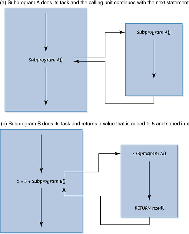
FIGURE 7.14 Subprogram flow of control
Recursive Factorial
The factorial of a number is defined as the number multiplied by the product of all the numbers between itself and 0:
N! = N * (N 2 1)!
The factorial of 0 is 1. The size factor is the number for which we are calculating the factorial. We have a base case:
Factorial(0) is 1.
We also have a general case:
Factorial(N) is N * Factorial(N – 1).
An if statement can evaluate N to see if it is 0 (the base case) or greater than 0 (the general case). Because N is clearly getting smaller with each call, the base case is eventually reached.
Each time Factorial is called, the value of N gets smaller. The data being given each time is called the argument. What happens if the argument is a negative number? The subprogram just keeps calling itself until the run-time support system runs out of memory. This situation, which is called infinite recursion, is equivalent to an infinite loop.
Recursive Binary Search
Although we coded the binary search using a loop, the binary search algorithm sounds recursive. We stop when we find the item or when we know it isn’t there (base cases). We continue to look for the item in the section of the array where it will be if it is present at all. A recursive algorithm must be called from a nonrecursive algorithm as we did with the factorial algorithm. Here the subprogram needs to know the first and last indices within which it is searching. Instead of resetting first or last as we did in the iterative version, we simply call the algorithm again with the new values for first and last.
Quicksort
The Quicksort algorithm, developed by C. A. R. Hoare, is based on the idea that it is faster and easier to sort two small lists than one larger one. The name comes from the fact that, in general, Quicksort can sort a list of data elements quite rapidly. The basic strategy of this sort is “divide and conquer.”
If you were given a large stack of final exams to sort by name, you might use the following approach: Pick a splitting value, say L, and divide the stack of tests into two piles, A–L and M–Z. (Note that the two piles do not necessarily contain the same number of tests.) Then take the first pile and subdivide it into two piles, A–F and G–L. The A–F pile can be further broken down into A–C and D–F. This division process goes on until the piles are small enough to be easily sorted by hand. The same process is applied to the M–Z pile.
Eventually, all of the small, sorted piles can be stacked one on top of the other to produce a sorted set of tests. See FIGURE 7.15.
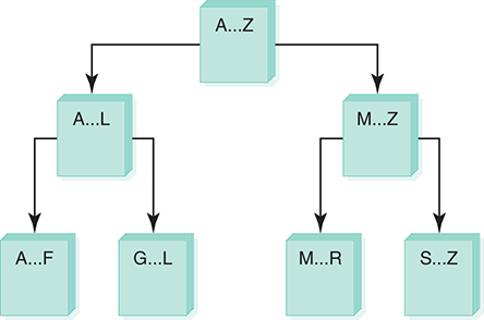
FIGURE 7.15 Ordering a list using the Quicksort algorithm
This strategy is based on recursion—on each attempt to sort the stack of tests, the stack is divided, and then the same approach is used to sort each of the smaller stacks (a smaller case). This process continues until the small stacks do not need to be divided further (the base case). The variables first and last in the Quicksort algorithm reflect the part of the array data that is currently being processed.
How do we select splitVal? One simple solution is to use whatever value is in data[first] as the splitting value. Let’s look at an example using data[first] as splitVal.
![An array of 8 numbers having splitVal equals 9 reads from [first] to [last], 9, 20, 6, 10, 14, 8, 60, and 11.](http://images-20200215.ebookreading.net/5/1/1/9781284155648/9781284155648__computer-science-illuminated__9781284155648__images__9781284156010_CH07_UN02.png)
After the call to Split, all items less than or equal to splitVal are on the left side of the array and all items greater than splitVal are on the right side of the array.
![An array of 8 numbers from [first] to [last] reads, 9, 8, 6, 10, 14, 20, 60, and 11. The first three numbers are labeled smaller values, the last five numbers are labeled larger values, and the [splitPoint] is marked between both the values.](http://images-20200215.ebookreading.net/5/1/1/9781284155648/9781284155648__computer-science-illuminated__9781284155648__images__9781284156010_CH07_UN03.png)
The two “halves” meet at splitPoint, the index of the last item that is less than or equal to splitVal. Note that we don’t know the value of splitPoint until the splitting process is complete. We can then swap splitVal (data[first]) with the value at data[splitPoint].
![An array of 8 numbers from [first] to [last] reads, 6, 8, 9, 10, 14, 20, 60, and 11. The first three numbers are labeled smaller values, the last five numbers are labeled larger values, and the [splitPoint] is marked between both the values.](http://images-20200215.ebookreading.net/5/1/1/9781284155648/9781284155648__computer-science-illuminated__9781284155648__images__9781284156010_CH07_UN04.png)
Our recursive calls to Quicksort use this index (splitPoint) to reduce the size of the problem in the general case.
Quicksort(first, splitPoint – 1) sorts the left “half” of the array. Quicksort(splitPoint + 1, last) sorts the right “half” of the array. (The “halves” are not necessarily the same size.) splitVal is already in its correct position in data[splitPoint].
What is the base case? When the segment being examined has only one item, we do not need to go on. That is represented in the algorithm by the missing else statement. If there is only one value in the segment being sorted, it is already in its place.
We must find a way to get all elements that are equal to or less than splitVal on one side of splitVal and all elements that are greater than splitVal on the other side. We do this by moving a pair of the indexes from the ends toward the middle of the array, looking for items that are on the wrong side of the split value. When we find pairs that are on the wrong side, we swap them and continue working our way into the middle of the array.
Although we still have an abstract step, we can stop, because we have already expanded this abstract step in an earlier problem. This brings up a very important point: Never reinvent the wheel. An abstract step in one algorithm may have been solved previously either by you or by someone else. FIGURE 7.16 shows an example of this splitting algorithm.

FIGURE 7.16 Splitting algorithm
Quicksort is an excellent sorting approach if the data to be sorted is in random order. If the data is already sorted, however, the algorithm degenerates so that each split has just one item in it.
Recursion is a very powerful and elegant tool. Nevertheless, not all problems can easily be solved recursively, and not all problems that have an obvious recursive solution should be solved recursively. Even so, a recursive solution is preferable for many problems. If the problem statement logically falls into two cases (a base case and a general case), recursion is a viable alternative.