
18.3 Problems
Life is full of all kinds of problems. There are problems for which it is easy to develop and implement computer solutions. There are problems for which we can implement computer solutions, but we wouldn’t get the results in our lifetime. There are problems for which we can develop and implement computer solutions, provided we have enough computer resources. There are problems for which we can prove there are no solutions. Before we can look at these categories of problems, we must introduce a way of comparing algorithms.
Comparing Algorithms
As we have shown in previous chapters, there is more than one way to solve most problems. If you were asked for directions to Joe’s Diner (see FIGURE 18.2), you could give either of two equally correct answers:
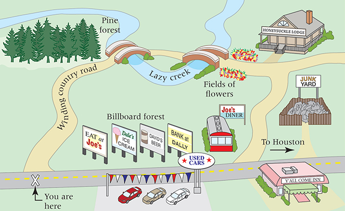
FIGURE 18.2 Equally valid solutions to the same problem
“Go east on the big highway to the Y’all Come Inn, and turn left.” or
“Take the winding country road to Honeysuckle Lodge, and turn right.”
The two answers are not the same, but because following either route gets the traveler to Joe’s Diner, both answers are functionally correct.
If the request for directions contained special requirements, one solution might be preferable to the other. For instance, “I’m late for dinner. What’s the quickest route to Joe’s Diner?” calls for the first answer, whereas “Is there a scenic road that I can take to get to Joe’s Diner?” suggests the second. If no special requirements are known, the choice is a matter of personal preference—which road do you like better?
Often the choice between algorithms comes down to a question of efficiency. Which one takes the least amount of computing time? Which one does the job with the least amount of work? Here we are interested in the amount of work that the computer does.
To compare the work done by competing algorithms, we must first define a set of objective measures that can be applied to each algorithm. The analysis of algorithms is an important area of theoretical computer science; in advanced computing courses, students see extensive work in this area. We cover only a small part of this topic in this book—just enough to allow you to compare two algorithms that do the same task and understand that the complexity of algorithms forms a continuum from easy to unsolvable.
How do programmers measure the work that two algorithms perform? The first solution that comes to mind is simply to code the algorithms and then compare the execution times for running the two programs. The one with the shorter execution time is clearly the better algorithm. Or is it? Using this technique, we really can determine only that program A is more efficient than program B on a particular computer. Execution times are specific to a particular computer. Of course, we could test the algorithms on all possible computers, but we want a more general measure.
A second possibility is to count the number of instructions or statements executed. This measure, however, varies with the programming language used as well as with the style of the individual programmer. To standardize this measure somewhat, we could count the number of passes through a critical loop in the algorithm. If each iteration involves a constant amount of work, this measure gives us a meaningful yardstick of efficiency.
Another idea is to isolate a particular operation fundamental to the algorithm and then count the number of times that this operation is performed. Suppose, for example, that we are summing the elements in an integer list. To measure the amount of work required, we could count the integer addition operations. For a list of 100 elements, there are 99 addition operations. Note that we do not actually have to count the number of addition operations; it is some function of the number of elements (N) in the list. Therefore, we can express the number of addition operations in terms of N: for a list of N elements, there are N 2 1 addition operations. Now we can compare the algorithms for the general case, not just for a specific list size.
Big-O Analysis
We have been talking about work as a function of the size of the input to the operation (for instance, the number of elements in the list to be summed). We can express an approximation of this function using a mathematical notation called order of magnitude, or Big-O notation. (This is the letter O, not a zero.) The order of magnitude of a function is identified with the term in the function that increases fastest relative to the size of the problem. For instance, if
f(N) = N4 + 100N2 + 10N + 50
then f(N) is of order N4—or, in Big-O notation, O(N4). That is, for large values of N, some multiple of N4 dominates the function for sufficiently large val ues of N. It isn’t that 100N2 + 10N + 50 is not important, it is just that as N gets larger, all other factors become irrelevant because the N4 term dominates.
How is it that we can just drop the low-order terms? Well, suppose you needed to buy an elephant and a goldfish from one of two pet suppliers. You really need only to compare the prices of elephants, because the cost of the goldfish is trivial in comparison (see FIGURE 18.3). In analyzing algorithms, the term that increases most rapidly relative to the size of the problem dominates the function, effectively relegating the others to the “noise” level. The cost of an elephant is so much greater that we could just ignore the goldfish. Similarly, for large values of N, N4 is so much larger than 50, 10N, or even 100N2 that we can ignore these other terms. This doesn’t mean that the other terms do not contribute to the computing time; it simply means that they are not significant in our approximation when N is “large.”

FIGURE 18.3 The price of a goldfish pales in comparison to the price of an elephant
What is this value N? N represents the size of the problem. Most problems involve manipulating data structures like those discussed in Chapter 8. As we already know, each structure is composed of elements. We develop algorithms to add an element to the structure and to modify or delete an element from the structure. We can describe the work done by these operations in terms of N, where N is the number of elements in the structure.
Suppose that we want to write all the elements in a list into a file. How much work does that task require? The answer depends on how many elements are in the list. Our algorithm is
If N is the number of elements in the list, the “time” required to do this task is
time-to-open-the-file + [N * (time-to-get-one-element + time-to-write-one-element)]
This algorithm is O(N) because the time required to perform the task is proportional to the number of elements (N)—plus a little to open the file. How can we ignore the open time in determining the Big-O approximation? Assuming that the time necessary to open a file is constant, this part of the algorithm is our goldfish. If the list has only a few elements, the time needed to open the file may seem significant. For large values of N, however, writing the elements is an elephant in comparison with opening the file.
The order of magnitude of an algorithm does not tell us how long in microseconds the solution takes to run on our computer. Sometimes we may need that kind of information. For instance, suppose a word processor’s requirements state that the program must be able to spell-check a 50-page document (on a particular computer) in less than 120 seconds. For this kind of information, we do not use Big-O analysis; we use other measurements. We can compare different implementations of a data structure by coding them and then running a test, recording the time on the computer’s clock before and after we conduct the test. This kind of “benchmark” test tells us how long the operations take on a particular computer, using a particular compiler. The Big-O analysis, by contrast, allows us to compare algorithms without reference to these factors.
Common Orders of Magnitude
O(1) is called bounded time.
The amount of work is bounded by a con stant and is not dependent on the size of the problem. Assigning a value to the ith element in an array of N elements is O(1), because an element in an array can be accessed directly through its index. Although bounded time is often called constant time, the amount of work is not necessarily constant. It is, however, bounded by a constant.
O(log2N) is called logarithmic time.
The amount of work depends on the log of the size of the problem. Algorithms that successively cut the amount of data to be processed in half at each step typically fall into this category. Finding a value in a list of sorted elements using the binary search algorithm is O(log2N).
O(N) is called linear time.
The amount of work is some constant times the size of the problem. Printing all of the elements in a list of N elements is O(N). Searching for a particular value in a list of unsorted elements is also O(N) because you (potentially) must search every element in the list to find it.
O(N log2N) is called (for lack of a better term) N log2N time.
Algorithms of this type typically involve applying a logarithmic algorithm N times. The better sorting algorithms, such as Quicksort, Heapsort, and Merge-sort, have N log2N complexity. That is, these algorithms can transform an unsorted list into a sorted list in O(N log2N) time, although Quicksort degenerates to O(N2) under certain input data.
O(N2) is called quadratic time.
Algorithms of this type typically involve applying a linear algorithm N times. Most simple sorting algorithms are O(N2) algorithms.
O(2N) is called exponential time.
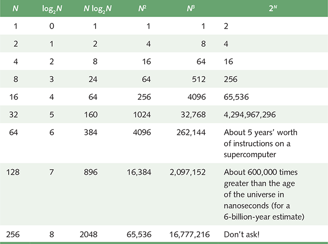
These algorithms are costly. As you can see in TABLE 18.2, exponential times increase dramatically in relation to the size of N. The fable of the King and the Corn demonstrates an exponential time algorithm, where the size of the problem is a kernel of corn. (The values in the last column of Table 18.2 grow so quickly that the computation time required for problems of this order may exceed the estimated life span of the universe!)
| TABLE | |
| 18.2 Comparison of rates of growth | |
|
|
O(N!) is called factorial time.
These algorithms are even more costly than exponential algorithms. The traveling salesperson graph algorithm (see page 618) is a factorial time algorithm.
Algorithms whose order of magnitude can be expressed as a polynomial in the size of the problem are called polynomial-time algorithms. Recall from Chapter 2 that a polynomial is a sum of two or more algebraic terms, each of which consists of a constant multiplied by one or more variables raised to a nonnegative integral power. Thus, polynomial algorithms are those whose order of magnitude can be expressed as the size of the problem to a power, and the Big-O complexity of the algorithm is the highest power in the polynomial. All polynomial-time algorithms are defined as being in Class P.
Think of common orders of complexity as being bins into which we sort algorithms (see FIGURE 18.4). For small values of the size of the problem, an algorithm in one bin may actually be faster than the equivalent algorithm in the next-more-efficient bin. As the size increases, the difference among algorithms in the different bins gets larger. When choosing between algorithms in the same bin, we look at the goldfish that we ignored earlier.
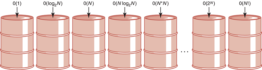
FIGURE 18.4 Orders of complexity
Turing Machines
We have mentioned Alan Turing several times in this book. He developed the concept of a computing machine in the 1930s. He was not interested in implementing his machine; rather, he used it as a model to study the limits of what can be computed.
A Turing machine, as his model became known, consists of a control unit with a read/write head that can read and write symbols on an infinite tape. The tape is divided into cells. The model is based on a person doing a primitive calculation on a long strip of paper using a pencil with an eraser. Each line (cell) of the paper contains a symbol from a finite alphabet. Starting at one cell, the person examines the symbol and then either leaves the symbol alone or erases it and replaces it with another symbol from the alphabet. The person then moves to an adjacent cell and repeats the action.
The control unit simulates the person. The human’s decision-making process is represented by a finite series of instructions that the control unit can execute. Each instruction causes:
■ A symbol to be read from a cell on the tape
■ A symbol to be written into the cell
■ The tape to be moved one cell left, moved one cell right, or remain positioned as it was
If we allow the person to replace a symbol with itself, these actions do, indeed, model a person with a pencil. See FIGURE 18.5.

FIGURE 18.5 Turing machine processing
Why is such a simple machine (model) of any importance? It is widely accepted that anything that is intuitively computable can be computed by a Turing machine. This statement is known as the Church–Turing thesis, named for Turing and Alonzo Church, another mathematician who developed a similar model known as the lambda calculus and with whom Turing worked at Princeton. The works of Turing and Church are covered in depth in theoretical courses in computer science.
It follows from the Church–Turing thesis that if we can find a problem for which a Turing-machine solution can be proven not to exist, then that problem must be unsolvable. In the next section we describe such a problem.
Halting Problem
It is not always obvious that a computation (program) halts. In Chapter 6, we introduced the concept of repeating a process; in Chapter 7, we talked about different types of loops. Some loops clearly stop, some loops clearly do not (infinite loops), and some loops stop depending on input data or calculations that occur within the loop. When a program is running, it is difficult to know whether it is caught in an infinite loop or whether it just needs more time to run.
It would be very beneficial if we could predict that a program with a specified input would not go into an infinite loop. The halting problem restates the question this way: Given a program and an input to the program, determine if the program will eventually stop with this input.
The obvious approach is to run the program with the specified input and see what happens. If it stops, the answer is clear. What if it doesn’t stop? How long do you run the program before you decide that it is in an infinite loop? Clearly, this approach has some flaws. Unfortunately, there are flaws in every other approach as well. This problem is unsolvable. Let’s look at the outlines of a proof of this assertion, which can be rephrased as follows: “There is no Turing-machine program that can determine whether a program will halt given a particular input.”
How can we prove that a problem is unsolvable or, rather, that we just haven’t found the solution yet? We could try every proposed solution and show that every one contains an error. Because there are many known solutions and many yet unknown, this approach seems doomed to failure. Yet, this approach forms the basis of Turing’s solution to this problem. In his proof, he starts with any proposed solution and then shows that it doesn’t work.
Assume that there exists a Turing-machine program called SolvesHaltingProblem that determines for any program Example and input SampleData whether program Example halts given input SampleData. That is, SolvesHaltingProblem takes program Example and SampleData and prints “Halts” if the program halts and “Loops” if the program contains an infinite loop. This situation is depicted in FIGURE 18.6.
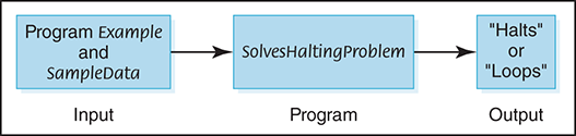
FIGURE 18.6 Proposed program for solving the halting problem
Recall that both programs (instructions) and data look alike in a computer; they are just bit patterns. What distinguishes programs from data is how the control unit interprets the bit pattern. So we could give program Example a copy of itself as data in place of SampleData. Thus SolvesHaltingProblem should be able to take program Example and a second copy of program Example as data and determine whether program Example halts with itself as data. See FIGURE 18.7.
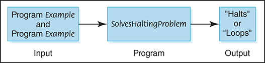
FIGURE 18.7 Proposed program for solving the halting problem
Now let’s construct a new program, NewProgram, that takes program Example as both program and data and uses the algorithm from SolvesHaltingProblem to write “Halts” if Example halts and “Loops” if it does not halt. If “Halts” is written, NewProgram creates an infinite loop; if “Loops” is written, NewProgram writes “Halts.” FIGURE 18.8 shows this situation.
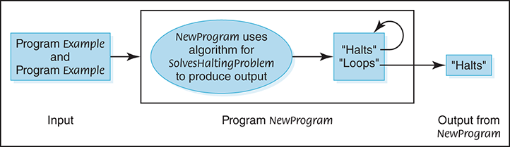
FIGURE 18.8 Construction of NewProgram
Do you see where the proof is leading? Let’s now apply program SolvesHaltingProblem to NewProgram, using NewProgram as data. If SolvesHaltingProblem prints “Halts,” program NewProgram goes into an infinite loop. If SolvesHaltingProblem prints “Loops,” program NewProgram prints “Halts” and stops. In either case, SolvesHaltingProblem gives the wrong answer. Because SolvesHaltingProblem gives the wrong answer in at least one case, it doesn’t work on all cases. Therefore, any proposed solution must have a flaw.
Classification of Algorithms
Figure 18.4 shows the common orders of magnitude as bins. We now know that there is another bin to the right, which would contain algorithms that are unsolvable. Let’s reorganize our bins a little, combining all polynomial algorithms in a bin labeled Class P. Then let’s combine exponential and factorial algorithms into one bin and add a bin labeled Unsolvable. See FIGURE 18.9.
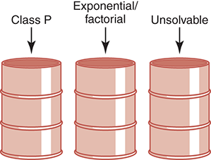
FIGURE 18.9 A reorganization of algorithm classifications
The algorithms in the middle bin have known solutions, but they are called intractable because for data of any size, they simply take too long to execute. We mentioned parallel computers in Chapter 1 when we reviewed the history of computer hardware. Could some of these problems be solved in a reasonable time (polynomial time) if enough processors worked on the problem at the same time? Yes, they could. A problem is said to be in Class NP if it can be solved with a sufficiently large number of processors in polynomial time.
Clearly, Class P problems are also in Class NP. An open question in theoretical computing is whether Class NP problems, whose only tractable solution is with many processors, are also in Class P. That is, do there exist polynomial-time algorithms for these problems that we just haven’t discovered (invented) yet? We don’t know, but the problem has been and is still keeping computer science theorists busy looking for the solution. The solution? Yes, the problem of determining whether Class P is equal to Class NP has been reduced to finding a solution for one of these algorithms. A special class called NP-complete problems is part of Class NP; these problems have the property that they can be mapped into one another. If a polynomial-time solution with one processor can be found for any one of the algorithms in this class, a solution can be found for each of them—that is, the solution can be mapped to all the others. How and why this is so is beyond the scope of this book. However, if the solution is found, you will know, because it will make headlines all over the computing world.
For now we picture our complexity bins with a new companion—a bin labeled Class NP. This bin and the Class P bin have dotted lines on their adjacent sides, because they may actually be just one bin. See FIGURE 18.10.
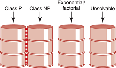
FIGURE 18.10 Adding Class NP
SUMMARY
Limits are imposed on computer problem-solving by the hardware, the software, and the nature of the problems to be solved. Numbers are infinite, but their representation within a computer is finite. This limitation can cause errors to creep into arithmetic calculations, giving incorrect results. Hardware components can wear out, and information can be lost during intercomputer and intracomputer data transfers.
The sheer size and complexity of large software projects almost guarantee that errors will occur. Testing a program can demonstrate errors, but it cannot prove the absence of errors. The best way to build good software is to pay attention to quality from the first day of the project, applying the principles of software engineering.
Problems vary from those that are very simple to solve to those that cannot be solved at all. Big-O analysis provides a metric that allows us to compare algorithms in terms of the growth rate of a size factor in the algorithm. Polynomial-time algorithms are those algorithms whose Big-O complexity can be expressed as a polynomial in the size factor. Class P problems can be solved with one processor in polynomial time. Class NP problems can be solved in polynomial time with an unlimited number of processors. As proved by Turing, the halting problem does not have a solution.
KEY TERMS
EXERCISES
For Exercises 1–15, match the Big-O notation with its definition or use.
O(1)
O(log2N)
O(N)
O(N log2N)
O(N2)
O(2N)
O(N!)
For Exercises 16–20, match the name of the technique with the algorithm.
Even parity
Odd parity
Check digits
Error-correcting codes
Parity bit
For Exercises 21–30, mark the answers true or false as follows:
True
False
Exercises 31–61 are problems or short-answer questions.
THOUGHT QUESTIONS
-
2. Search the Web for the answers to the following questions.
Did the Russian Phobos 1 spacecraft commit suicide?
What caused the delay in the opening of the Denver airport?
What was the cost of the software repair in London’s ambulance dispatch system failure?
The USS Yorktown was dead in the water for several hours in 1998. What software error caused the problem?