
10.4 CPU Scheduling
CPU scheduling is the act of determining which process in the ready state should be moved to the running state. That is, CPU-scheduling algorithms decide which process should be given over to the CPU so that it can make computational progress.
CPU-scheduling decisions are made when a process switches from the running state to the waiting state, or when a program terminates. This type of CPU scheduling is called nonpreemptive scheduling, because the need for a new CPU process results from the activity of the currently executing process.
CPU-scheduling decisions may also be made when a process moves from the running state to the ready state or when a process moves from the waiting state to the ready state. These are examples of preemptive scheduling, because the currently running process (through no fault of its own) is preempted by the operating system.
Scheduling algorithms are often evaluated using metrics, such as the turnaround time for a process. This measure is the amount of time between when a process arrives in the ready state and when it exits the running state for the last time. We would like, on average, for the turnaround time for our processes to be small.
Several different approaches can be used to determine which process gets chosen first to move from the ready state to the running state. We examine three of them in the next sections.
First Come, First Served
In the first-come, first-served (FCFS) scheduling approach, processes are moved to the CPU in the order in which they arrive in the running state. FCFS scheduling is nonpreemptive. Once a process is given access to the CPU, it keeps that access unless it makes a request that forces it to wait, such as a request for a device in use by another process.
Suppose processes p1 through p5 arrive in the ready state at essentially the same time (to make our calculations simple) but in the following order and with the specified service time:
| Process | Service Time |
| p1 | 140 |
| p2 | 75 |
| p3 | 320 |
| p4 | 280 |
| p5 | 125 |
In the FCFS scheduling approach, each process receives access to the CPU in turn. For simplicity, we assume here that processes don’t cause themselves to wait. The following Gantt chart shows the order and time of process completion:

Because we are assuming the processes all arrived at the same time, the turnaround time for each process is the same as its completion time. The average turnaround time is (140 + 215 + 535 + 815 + 940) / 5 or 529.
In reality, processes do not arrive at exactly the same time. In this case, the calculation of the average turnaround time would be similar, but would take into account the arrival time of each process. The turnaround time for each process would be its completion time minus its arrival time.
The FCFS algorithm is easy to implement but suffers from its lack of attention to important factors such as service time requirements. Although we used the service times in our calculations of turnaround time, the algorithm didn’t use that information to determine the best order in which to schedule the processes.
Shortest Job Next
The shortest-job-next (SJN) CPU-scheduling algorithm looks at all processes in the ready state and dispatches the one with the smallest service time. Like FCFS, it is generally implemented as a nonpreemptive algorithm. Below is the Gantt chart for the same set of processes we examined in the FCFS example. Because the selection criteria are different, the order in which the processes are scheduled and completed are different:

The average turnaround time for this example is (75 + 200 + 340 + 620 + 940) / 5 or 435.
Note that the SJN algorithm relies on knowledge of the future. That is, it gives access to the CPU to the job that runs for the shortest time when it is allowed to execute. That time is essentially impossible to determine. Thus, to run this algorithm, the service time value for a process is typically estimated by the operating system using various probability factors and taking the type of job into account. If these estimates are wrong, the premise of the algorithm breaks down and its efficiency deteriorates. The SJN algorithm is provably optimal, meaning that if we could know the service time of each job, the algorithm would produce the shortest turnaround time for all jobs compared to any other algorithm. However, because we can’t know the future absolutely, we make guesses and hope those guesses are correct.
Round Robin
Round-robin CPU scheduling distributes the processing time equitably among all ready processes. This algorithm establishes a particular time slice (or time quantum), which is the amount of time each process receives before it is preempted and returned to the ready state to allow another process to take its turn. Eventually the preempted process will be given another time slice on the CPU. This procedure continues until the process gets all the time it needs to complete and terminates.
Note that the round-robin algorithm is preemptive. The expiration of a time slice is an arbitrary reason to remove a process from the CPU. This action is represented by the transition from the running state to the ready state.
Suppose the time slice used for a particular round-robin scheduling algorithm was 50 and we used the same set of processes as our previous examples. The Gantt chart results are:
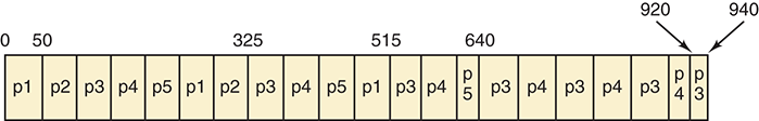
Each process is given a time slice of 50, unless it doesn’t need a full slice. For example, process 2 originally needed 75 time units. It was given an initial time slice of 50. When its turn to use the CPU came around again, it needed only 25 time units. Therefore, process 2 terminates and gives up the CPU at time 325.
The average turnaround time for this example is (515 + 325 + 940 + 920 + 640) / 5, or 668. This turnaround time is larger than the times in the other examples. Does that mean the round-robin algorithm is not as good as the other options? No. We can’t make such general claims based on one example. We can say only that one algorithm is better than another for that specific set of processes. General analysis of algorithm efficiencies is much more involved.
The round-robin CPU process scheduling algorithm is probably the most widely used. It generally supports all kinds of jobs and is considered the most fair.
SUMMARY
An operating system is the part of the system software that manages resources on a computer. It serves as moderator among human users, application software, and the hardware devices in the system.
Multiprogramming is the technique for keeping multiple programs in memory at the same time, contending for time on the CPU. A process is a program in execution. The operating system must perform careful CPU scheduling, memory management, and process management to ensure fair access to the CPU.
Batch processing organizes jobs into batches that use the same or similar resources. Timesharing allows multiple users to interact with a computer at the same time, creating a virtual machine for each user.
An operating system must manage memory to control and monitor where processes are loaded into main memory. Any memory management technique must define the manner in which it binds a logical address to a physical one. Various strategies have been developed for memory management. The single contiguous approach allows only one program other than the operating system to be in main memory. The partition approach divides memory into several partitions into which processes are loaded. Fixed partitions have a set size, whereas dynamic partitions are created to satisfy the unique needs of the processes loaded. Paging divides memory into frames and programs into pages. The pages of a program need not be contiguous in memory. Demand paging allows for only a portion of a program to be in memory at any given time.
An operating system manages a process’s life states, which are the stages a program goes through during its execution. The process control block stores the necessary information for any process.
CPU-scheduling algorithms determine which process gets priority to use the CPU next. First-come, first-served CPU scheduling gives priority to the earliest-arriving job. The shortest-job-next algorithm gives priority to jobs with short running times. Round-robin scheduling rotates the CPU among active processes, giving a little time to each process.
KEY TERMS
EXERCISES
For Exercises 1–18, mark the answers true or false as follows:
True
False
For Exercises 19–23, match the operating system with information about it.
Mac OS
UNIX
Linux
DOS
Windows
For Exercises 24–26, match the following software type with its definition.
Systems software
Operating system
Application software
Exercises 27–72 are problems or short-answer questions.
-
36. In Chapter 6, we defined a virtual machine as a hypothetical machine designed to illustrate important features of a real machine. In this chapter, we define a virtual machine as the illusion created by a timesharing system that each user has a dedicated machine. Relate these two definitions.
Exercises 55 and 56 use the following state of memory.

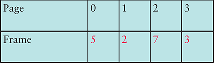
Exercises 58–60 refer to the following PMT.
Use the following table of processes and service time for Exercises 69 through 72.

THOUGHT QUESTIONS
-
1. In Chapter 5, we said that the control unit was like the stage manager who organized and managed the other parts of the von Neumann machine. Suppose we now say the operating system is also like a stage manager, but on a much grander scale. Does this analogy hold or does it break down?
-
2. The user interface that the operating system presents to the user is like a hallway with doors leading to rooms housing applications programs. To go from one room to another, you have to go back to the hallway. Continue with this analogy: What would files be? What would be analogous to a time slice?