
14.2 Specific Models
In this section, we examine three types of simulation models.
Queuing Systems
Let’s look at a very useful type of simulation called a queuing system. A queuing system is a discrete-event model that uses random numbers to represent the arrival and duration of events. A queuing system is made up of servers and queues of objects to be served. Recall from Chapter 8 that a queue is a first-in, first-out (FIFO) structure. We deal with queuing systems all the time in our daily lives. When you stand in line to check out at the grocery store or to cash a check at the bank, you are dealing with a queuing system. When you submit a “batch job” (such as a compilation) on a mainframe computer, your job must wait in line until the CPU finishes the jobs scheduled ahead of it. When you make a phone call to reserve an airline ticket and get a recording (“Thank you for calling Air Busters; your call will be answered by the next available operator”), you are dealing with a queuing system.
Please Wait
Waiting is the critical element. The objective of a queuing system is to utilize the servers (the tellers, checkers, CPU, operators, and so on) as fully as possible while keeping the wait time within a reasonable limit. These goals usually require a compromise between cost and customer satisfaction.
To put this on a personal level, no one likes to stand in line. If there were one checkout counter for each customer in a supermarket, the customers would be delighted. The supermarket, however, would not be in business very long. So a compromise is made: The number of cashiers is kept within the limits set by the store’s budget, and the average customer is not kept waiting too long.
How does a company determine the optimal compromise between the number of servers and the wait time? One way is by experience— the company tries out different numbers of servers and sees how things work out. There are two problems with this approach: It takes too long and it is too expensive. Another way of examining this problem is to use a computer simulation.
To construct a queuing model, we must know the following four things:
The number of events and how they affect the system so we can determine the rules of entity interaction
The number of servers
The distribution of arrival times so we can determine if an entity enters the system
The expected service time so we can determine the duration of an event
The simulation uses these characteristics to predict the average wait time. The number of servers, the distribution of arrival times, and the duration of service can be changed. The average wait times are then examined to determine what a reasonable compromise would be.
An Example
Consider the case of a drive-through bank with one teller. How long does the average car have to wait? If business gets better and cars start to arrive more frequently, what would be the effect on the average wait time? When would the bank need to open a second drive-through window?
This problem has the characteristics of a queuing model. The entities are a server (the teller), the objects being served (the customers in cars), and a queue to hold the objects waiting to be served (customers in cars). The average wait time is what we are interested in observing. The events in this system are the arrivals and the departures of customers.
Let’s look at how we can solve this problem as a time-driven simulation. A time-driven simulation is one in which the model is viewed at uniform time intervals—say, every minute. To simulate the passing of a unit of time (a minute, for example), we increment a clock. We run the simulation for a predetermined amount of time—say, 100 minutes. (Of course, simulated time usually passes much more quickly than real time; 100 simulated minutes passes in a flash on the computer.)
Think of the simulation as a big loop that executes a set of rules for each value of the clock—from 1 to 100, in our example. Here are the rules that are processed in the loop body:
Rule 1. If a customer arrives, he or she gets in line.
Rule 2. If the teller is free and if there is anyone waiting, the first customer in line leaves the line and advances to the teller’s window. The service time is set for that customer.
Rule 3. If a customer is at the teller’s window, the time remaining for that customer to be serviced is decremented.
Rule 4. If there are customers in line, the additional minute that they have remained in the queue (their wait time) is recorded.
The output from the simulation is the average wait time. We calculate this value using the following formula:
Average wait time = total wait time for all customers ÷ number of customers
Given this output, the bank can see whether its customers have an unreasonable wait in a one-teller system. If so, the bank can repeat the simulation with two tellers.
Not so fast! There are still two unanswered questions. How do we know if a customer arrived? How do we know when a customer has finished being serviced? We must provide the simulation with data about the arrival times and the service times, both of which are variables (parameters) in the simulation. We can never predict exactly when a customer will arrive or how long each individual customer will take. We can, however, make educated guesses, such as a customer arrives about every five minutes and most customers take about three minutes to service.
How do we know whether a job has arrived in this particular clock unit? The answer is a function of two factors: the number of minutes between arrivals (five in this case) and chance. Chance? Queuing models are based on chance? Well, not exactly. Let’s express the number of minutes between arrivals another way—as the probability that a job arrives in any given clock unit. Probabilities range from 0.0 (no chance) to 1.0 (a sure thing). If on average a new job arrives every five minutes, then the chance of a customer arriving in any given minute is 0.2 (1 chance in 5). Therefore, the probability of a new customer arriving in a particular minute is 1.0 divided by the number of minutes between arrivals.
Now what about luck? In computer terms, luck can be represented by the use of a random-number generator. We simulate the arrival of a customer by writing a function that generates a random number between 0.0 and 1.0 and applies the following rules:
If the random number is between 0.0 and the arrival probability, a job has arrived.
If the random number is greater than the arrival probability, no job arrived in this clock unit.
By changing the rate of arrival, we simulate what happens with a one-teller system where each transaction takes about three minutes as more and more cars arrive. We can also have the duration of service time based on probability. For example, we could simulate a situation where 60% of the people require three minutes, 30% of the people require five minutes, and 10% of the people require ten minutes.
Simulation doesn’t give us the answer or even an answer. Simulation is a technique for trying out “what if” questions. We build the model and run the simulation many times, trying various combinations of the parameters and observing the average wait time. What happens if the cars arrive more quickly? What happens if the service time is reduced by 10%? What happens if we add a second teller?
Other Types of Queues
The queue in the previous example was a FIFO queue: The entity that receives service is the entity that has been in the queue the longest time. Another type of queue is a priority queue. In a priority queue, each item in the queue is associated with a priority. When an item is dequeued, the item returned is the one with the highest priority. A priority queue operates like triage in the medical field. When multiple injured or ill people arrive at the same time, the doctors determine the severity of each person’s injuries. Those with the most severe problems get treated first.
Another scheme for ordering events is to have two FIFO queues: one for short service times and one for longer service times. This scheme is similar to the express lane at the supermarket. If you have fewer than ten items, you can go into the queue for the express lane; otherwise, you must enter the queue for one of the regular lanes.
Meteorological Models
In the last section we looked at a fairly simple simulation with discrete inputs and outputs. We now jump to a discussion of a continuous simulation: predicting the weather. The details of weather prediction are over the heads of all but professional meteorologists. In general, meteorological models are based on the time-dependent partial differential equations of fluid mechanics and thermodynamics. Equations exist for horizontal wind velocity components, the vertical velocity, temperature, pressure, and water vapor concentration. A few such equations are shown in FIGURE 14.1. Don’t worry, working with these equations is beyond the scope of this book—we just want to convey some of the complex processing that occurs in these types of models.
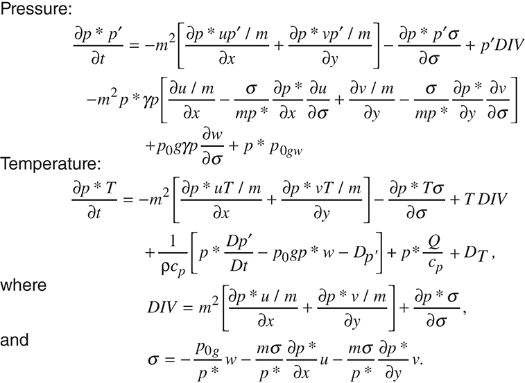
FIGURE 14.1 Some of the complex equations used in meteorological models
To predict the weather, initial values for the variables are entered from observation, and then the equations are solved to identify the values of the variables at some later time.4 These results are then reintegrated using the predicted values as the initial conditions. This process of reintegrating using the predicted values from that last integration as the observed values for the current integration continues, giving the predictions over time. Because these equations describe rates of change of entities in the model, the answers after each solution give values that can be used to predict the next set of values.
These types of simulation models are computationally expensive. Given the complexity of the equations and the fact that they must hold true at each point in the atmosphere, high-speed parallel computers are needed to solve them in a reasonable amount of time.
Weather Forecasting
“Red sky in the morning, sailor take warning” is an often-quoted weather prediction. Before the advent of computers, weather forecasting was based on folklore and observations. In the early 1950s, the first computer models were developed for weather forecasting. These models took the form of very complex sets of partial differential equations. As computers grew in size, the weather forecasting models grew even more complex.
If weathercasters use computer models to predict the weather, why are TV or radio weathercasts in the same city different? Why are they sometimes wrong? Computer models are designed to aid the weather-caster, not replace him or her. The outputs from the computer models are predictions of the values of variables in the future. It is up to the weathercaster to determine what the values mean.
Note that in the last paragraph we referred to multiple models. Different models exist because they make different assumptions. However, all computer models approximate the earth’s surface and the atmosphere above the surface using evenly spaced grid points. The distance between these points determines the size of the grid boxes, or resolution. The larger the grid boxes, the poorer the model’s resolution becomes. The Nested Grid model (NGM) has a horizontal resolution of 80 km and 18 vertical levels, and views the atmosphere as divided into squares for various levels of the atmosphere. Grids with smaller squares are nested inside larger ones to focus on particular geographic areas. The NGM forecasts 0–48 hours into the future every 6 hours.
The Model Output Statistics (MOS) model consists of a set of statistical equations tailored to various cities in the United States. The ETA model, named after the ETA coordinate system that takes topographical features such as mountains into account, is a newer model that closely resembles the NGM but has better resolution (29 km).5 WRF is an extension of ETA, which uses a variable-size grid of 4 to 12.5, and 25 to 37 levels.
The output from weather models can be in text form or graphical form. The weathercaster’s job is to interpret all of the output. But any good weathercaster knows that the output from any of these models is only as good as the input used as a starting point for the differential equations. This data comes from a variety of sources, including radiosondes (to measure humidity, temperature, and pressure at high altitudes), rawinsondes (to measure wind velocity aloft), aircraft observations, surface observations, satellites, and other remote sensing sources. A small error in any of the input variables can cause an increasing error in the values as the equations are reintegrated over time. Another problem is that of scale. The resolution of a model may be too coarse for the weathercaster to accurately interpret the results within his or her immediate area.
Different weathercasters may believe the predictions or may decide that other factors indicate that the predictions are in error. In addition, the various models may give conflicting results. It is up to the weather-caster to make a judgment as to which, if any, is correct.
Hurricane Tracking
The modules for hurricane tracking are called relocatable models, because they are applied to a moving target. That is, the geographical location of the model’s forecast varies from run to run (that is, from hurricane to hurricane). The Geophysical and Fluid Dynamics Laboratory (GFDL) developed the most recent hurricane model in an effort to improve the prediction of where a hurricane would make landfall.
The GFDL hurricane model became operational in 1995. The equations were such that the forecasts couldn’t be made fast enough to be useful until the National Weather Service’s high-performance supercomputers were used in parallel operation, which increased the running time over the serial implementation by 18%. FIGURE 14.2 shows the improvement of this model over the previous ones used to track hurricanes.
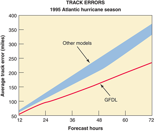
FIGURE 14.2 Improvements in hurricane models
Reprinted, by permission, from the National Science and Technology Council, High Performance Computing and Communications: Advancing the Frontiers of Information Technology
GFDL is being replaced by a specialized version of WRF, called HWRF. HWRF uses 27- and 9-km grid cells with 42 levels. It also takes information from a second simulation called the Princeton Ocean Model, which provides data on ocean currents and temperatures.
Some researchers are producing models that combine the outputs of other models. Such combined models, which have been called “superensembles,” give better results than individual models. The longer this kind of model runs, the better its results are. In one study focusing on a forecast of hurricane winds three days into the future, a combined model had an error of 21.5 mph as compared to the individual model errors that ranged from 31.3 mph to 32.4 mph.
Specialized Models
Meteorological models can be adapted and specialized for research purposes. For example, numeric-model simulations of atmospheric processes are being combined with air-chemistry models to diagnose atmospheric transport and diffusion for a variety of air-quality applications. One such study analyzed the part played by the topography of the Grand Canyon region of Arizona in the movement of air pollution.
Another study showed that by assimilating or ingesting observed data within the model solution as the model was running forward in time, rather than using observations at only the initial time, the model’s performance increased significantly. This allows for improved numerical representations of the atmosphere for input into other specialized models.6
Advanced meteorological modeling systems can be used to provide guidance for other complex systems in the military or aviation industry. For example, the weather has an impact on projectile motions and must be taken into consideration in battlefield situations. In the aviation industry, meteorological data is used in diverse ways, from determining how much fuel to carry to deciding when to move planes to avoid hail damage.
Computational Biology
Computational biology is an interdisciplinary field that applies techniques of computer science, applied mathematics, and statistics to problems in biology. These techniques include model building, computer simulation, and graphics. Much biological research, including genetic/genomic research, is now conducted via computational techniques and modeling rather than in traditional “wet” laboratories with chemicals. Computational tools enabled genomic researchers to map the complete human genome by 2003; using traditional sequencing methods would have required many more years to accomplish this objective. Computational techniques have also assisted researchers in locating the genes for many diseases, which has resulted in pharmaceuticals being developed to treat and cure those diseases.
Computational biology encompasses numerous other fields, including the following:
Bioinformatics, the application of information technology to molecular biology. It involves the acquisition, storage, manipulation, analyses, visualization, and sharing of biological information on computers and computer networks.
Computational biomodeling, the building of computational models of biological systems.
Computational genomics, the deciphering of genome sequences.
Molecular modeling, the modeling of molecules.
Protein structure prediction, the attempt to produce models of three-dimensional protein structures that have yet to be found experimentally.
Other Models
In a sense, every computer program is a simulation, because a program represents the model of the solution that was designed in the problem-solving phase. When the program is executed, the model is simulated. We do not wish to go down this path, however, for this section would become infinite. There are, however, several disciplines that explicitly make use of simulation.
Will the stock market go higher? Will consumer prices rise? If we increase the money spent on advertising, will sales go up? Forecasting models help to answer these questions. However, these forecasting models are different from those used in weather forecasting. Weather models are based on factors whose interactions are mostly known and can be modeled using partial differential equations of fluid mechanics and thermo dynamics. Business and economic forecasting models are based on past history of the variables involved, so they use regression analysis as the basis for prediction.
Seismic models depict the propagation of seismic waves through the earth’s medium. These seismic waves can come from natural events, such as earthquakes and volcanic eruptions, or from human-made events, such as controlled explosions, reservoir-induced earthquakes, or cultural noise (industry or traffic). For natural events, sensors pick up the waves. Models, using these observations as input, can then determine the cause and magnitude of the source causing the waves. For human-made events, given the size of the event and the sensor data, models can map the earth’s subsurface. Such models may be used to explore for oil and gas. The seismic data is used to provide geologists with highly detailed three-dimensional maps of hidden oil and gas reservoirs before drilling begins, thereby minimizing the possibility of drilling a dry well.
Computing Power Necessary
Many of the equations necessary to construct the continuous models discussed here were developed many years ago. That is, the partial differential equations that defined the interactions of the entities in the model were known. However, the models based on them could not be simulated in time for the answers to be useful. The introduction of parallel high-performance computing in the mid-1990s changed all that. Newer, bigger, faster machines allow scientists to solve more complex mathematical systems over larger domains and ever-finer grids with even shorter wall clock times. The new machines are able to solve the complex equations fast enough to provide timely answers. Numerical weather forecasting, unlike some other applications, must beat the clock. After all, yesterday’s weather prediction is not very useful if it is not received until today.