
1.6 Substitution Methods and Exact Equations
The first-order differential equations we have solved in the previous sections have all been either separable or linear. But many applications involve differential equations that are neither separable nor linear. In this section we illustrate (mainly with examples) substitution methods that sometimes can be used to transform a given differential equation into one that we already know how to solve.
For instance, the differential equation
with dependent variable y and independent variable x, may contain a conspicuous combination
of x and y that suggests itself as a new independent variable v. Thus the differential equation
practically demands the substitution v=x+y+3
If the substitution relation in Eq. (2) can be solved for
then application of the chain rule—regarding v as an (unknown) function of x—yields
where the partial derivatives ∂β/∂x=βx(x,v)
with new dependent variable v. If this new equation is either separable or linear, then we can apply the methods of preceding sections to solve it.
If v=v(x)
Example 1
Solve the differential equation
Solution
As indicated earlier, let’s try the substitution
Then
so the transformed equation is
This is a separable equation, and we have no difficulty in obtaining its solution
So v=tan(x−C)
Remark
Figure 1.6.1 shows a slope field and typical solution curves for the differential equation of Example 1. We see that, although the function f(x,y)=(x+y+3)2

FIGURE 1.6.1.
Slope field and solution curves for y′=(x+y+3)2
Example 1 illustrates the fact that any differential equation of the form
can be transformed into a separable equation by use of the substitution v=ax+by+c
Homogeneous Equations
A homogeneous first-order differential equation is one that can be written in the form
![]()
If we make the substitutions
then Eq. (7) is transformed into the separable equation
Thus every homogeneous first-order differential equation can be reduced to an integration problem by means of the substitutions in (8).
Remark
A dictionary definition of “homogeneous” is “of a similar kind or nature.” Consider a differential equation of the form
whose polynomial coefficient functions are “homogeneous” in the sense that each of their terms has the same total degree, m+n=p+q=r+s=K
which evidently can be written (by another division) in the form of Eq. (7). More generally, a differential equation of the form P(x,y)y′=Q(x,y)
Example 2
Solve the differential equation
Solution
This equation is neither separable nor linear, but we recognize it as a homogeneous equation by writing it in the form
The substitutions in (8) then take the form
These yield
and hence
We apply the exponential function to both sides of the last equation to obtain
Note that the left-hand side of this equation is necessarily nonnegative. It follows that k>0

FIGURE 1.6.2.
Slope field and solution curves for 2xyy′=4x2+3y2
Example 3
Solve the initial value problem
where x0>0
Solution
We divide both sides by x and find that
so we make the substitutions in (8); we get
We need not write ln |x|
and therefore
is the desired particular solution. Figure 1.6.3 shows some typical solution curves. Because of the radical in the differential equation, these solution curves are confined to the indicated triangular region x≧|y|.

FIGURE 1.6.3.
Solution curves for xy′=y+√x2−y2.
Bernoulli Equations
A first-order differential equation of the form
![]()
is called a Bernoulli equation. If either n=0
![]()
transforms Eq. (9) into the linear equation
Rather than memorizing the form of this transformed equation, it is more efficient to make the substitution in Eq. (10) explicitly, as in the following examples.
Example 4
If we rewrite the homogeneous equation 2xyy′=4x2+3y2
we see that it is also a Bernoulli equation with P(x)=−3/(2x), Q(x)=2x, n=−1
This gives
Then multiplication by 2v1/2
with integrating factor ρ=e∫(−3/x)dx=x−3
Example 5
The equation
is neither separable nor linear nor homogeneous, but it is a Bernoulli equation with n=43, 1−n=−13.
transform it into
Division by −3xv−4
with integrating factor ρ=e∫(−2/x)dx=x−2
and finally,
Example 6
The equation
is neither separable, nor linear, nor homogeneous, nor is it a Bernoulli equation. But we observe that y appears only in the combinations e2y
that transforms Eq. (11) into the linear equation xv′(x)=3x4+v(x)
After multiplying by the integrating factor ρ=1/x
and hence
Flight Trajectories
Suppose that an airplane departs from the point (a, 0) located due east of its intended destination—an airport located at the origin (0, 0). The plane travels with constant speed v0

FIGURE 1.6.4.
The airplane headed for the origin.
Figure 1.6.5 helps us derive the plane’s velocity components relative to the ground. They are
Hence the trajectory y=f(x)
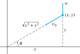
FIGURE 1.6.5.
The components of the velocity vector of the airplane.
If we set
the ratio of the windspeed to the plane’s airspeed, then Eq. (12) takes the homogeneous form
The substitution y=xv, y′=v+xv′ then leads routinely to
By trigonometric substitution, or by consulting a table for the integral on the left, we find that
and the initial condition v(a)=y(a)/a=0 yields
As we ask you to show in Problem 68, the result of substituting (17) in Eq. (16) and then solving for v is
Because y=xv, we finally obtain
for the equation of the plane’s trajectory.
Note that only in the case k<1 (that is, w<v0) does the curve in Eq. (19) pass through the origin, so that the plane reaches its destination. If w=v0 (so that k=1), then Eq. (19) takes the form y(x)=12a(1−x2/a2), so the plane’s trajectory approaches the point (0, a/2) rather than (0, 0). The situation is even worse if w>v0 (so k>1)-in this case it follows from Eq. (19) that y→+∞ as x→0. The three cases are illustrated in Fig. 1.6.6.

FIGURE 1.6.6.
The three cases w<v0 (plane velocity exceeds wind velocity), w=v0 (equal velocities), and w>v0 (wind is greater).
Example 7
Flight trajectory If a=200 mi, v0=500 mi/h, and w=100 mi/h, then k=w/v0=15, so the plane will succeed in reaching the airport at (0, 0). With these values, Eq. (19) yields
Now suppose that we want to find the maximum amount by which the plane is blown off course during its trip. That is, what is the maximum value of y(x) for 0≦x≦200?
Solution
Differentiation of the function in Eq. (20) yields
and we readily solve the equation y′(x)=0 to obtain (x/200)2/5=23. Hence
Thus the plane is blown almost 15 mi north at one point during its westward journey. (The graph of the function in Eq. (20) is the one used to construct Fig. 1.6.4. The vertical scale there is exaggerated by a factor of 4.)
Exact Differential Equations
We have seen that a general solution y(x) of a first-order differential equation is often defined implicitly by an equation of the form
where C is a constant. On the other hand, given the identity in (21), we can recover the original differential equation by differentiating each side with respect to x. Provided that Eq. (21) implicitly defines y as a differentiable function of x, this gives the original differential equation in the form
that is,
where M(x,y)=Fx(x,y) and N(x,y)=Fy(x,y).
It is sometimes convenient to rewrite Eq. (22) in the more symmetric form
![]()
called its differential form. The general first-order differential equation y′=f(x,y) can be written in this form with M=f(x,y) and N≡−1. The preceding discussion shows that, if there exists a function F(x,y) such that
then the equation
![]()
implicitly defines a general solution of Eq. (23). In this case, Eq. (23) is called an exact differential equation—the differential
of F(x,y) is exactly M dx+N dy.
Natural questions are these: How can we determine whether the differential equation in (23) is exact? And if it is exact, how can we find the function F such that Fx=M and Fy=N? To answer the first question, let us recall that if the mixed second-order partial derivatives Fxy and Fyx are continuous on an open set in the xy-plane, then they are equal: Fxy=Fyx. If Eq. (23) is exact and M and N have continuous partial derivatives, it then follows that
Thus the equation
![]()
is a necessary condition that the differential equation M dx+N dy=0 be exact. That is, if My≠Nx, then the differential equation in question is not exact, so we need not attempt to find a function F(x, y) such that Fx=M and Fy=N—there is no such function.
Example 8
The differential equation
is exact because we can immediately see that the function F(x,y)=xy3 has the property that Fx=y3 and Fy=3xy2. Thus a general solution of Eq. (25) is
if you prefer, y(x)=kx−1/3.
But suppose that we divide each term of the differential equation in Example 8 by y2 to obtain
This equation is not exact because, with M=y and N=3x, we have
Hence the necessary condition in Eq. (24) is not satisfied.
We are confronted with a curious situation here. The differential equations in (25) and (26) are essentially equivalent, and they have exactly the same solutions, yet one is exact and the other is not. In brief, whether a given differential equation is exact or not is related to the precise form M dx+N dy=0 in which it is written.
Theorem 1 tells us that (subject to differentiability conditions usually satisfied in practice) the necessary condition in (24) is also a sufficient condition for exactness. In other words, if My=Nx, then the differential equation M dx+N dy=0 is exact.
Proof:
We have seen already that it is necessary for Eq. (24) to hold if Eq. (23) is to be exact. To prove the converse, we must show that if Eq. (24) holds, then we can construct a function F(x, y) such that ∂F/∂x=M and ∂F/∂y=N. Note first that, for any function g(y), the function
satisfies the condition ∂F/∂x=M. (In Eq. (27), the notation ∫M(x, y)dx denotes an antiderivative of M(x, y) with respect to x.) We plan to choose g(y) so that
as well; that is, so that
To see that there is such a function of y, it suffices to show that the right-hand side in Eq. (28) is a function of y alone. We can then find g(y) by integrating with respect to y. Because the right-hand side in Eq. (28) is defined on a rectangle, and hence on an interval as a function of x, it suffices to show that its derivative with respect to x is identically zero. But
∂∂x(N−∂∂y∫M(x, y)dx)=∂N∂x−∂∂x∂∂y∫M(x, y)dx=∂N∂x−∂∂y∂∂x∫M(x, y)dx=∂N∂x−∂M∂y=0by hypothesis. So we can, indeed, find the desired function g(y) by integrating Eq. (28). We substitute this result in Eq. (27) to obtain
as the desired function with Fx=M and Fy=N.
Instead of memorizing Eq. (29), it is usually better to solve an exact equation M dx+N dy=0 by carrying out the process indicated by Eqs. (27) and (28). First we integrate M(x, y) with respect to x and write
thinking of the function g(y) as an “arbitrary constant of integration” as far as the variable x is concerned. Then we determine g(y) by imposing the condition that ∂F/∂y=N(x, y). This yields a general solution in the implicit form F(x, y)=C.
Example 9
Solve the differential equation
Solution
Let M(x, y)=6xy−y3 and N(x, y)=4y+3x2−3xy2. The given equation is exact because
Integrating ∂F/∂x=M(x, y) with respect to x, we get
Then we differentiate with respect to y and set ∂F/∂y=N(x, y). This yields
and it follows that g′(y)=4y. Hence g(y)=2y2+C1, and thus
Therefore, a general solution of the differential equation is defined implicitly by the equation
(we have absorbed the constant C1 into the constant C).
Remark
Figure 1.6.7 shows a rather complicated structure of solution curves for the differential equation of Example 9. The solution satisfying a given initial condition y(x0)=y0 is defined implicitly by Eq. (31), with C determined by substituting x=x0 and y=y0 in the equation. For instance, the particular solution satisfying y(0)=1 is defined implicitly by the equation 3x2y−xy3+2y2=2. The other two special points in the figure—at (0, 0) and near (0.75, 2.12)—are ones where both coefficient functions in Eq. (30) vanish, so the theorem of Section 1.3 does not guarantee a unique solution.

FIGURE 1.6.7.
Slope field and solution curves for the exact equation in Example 9.
Reducible Second-Order Equations
A second-order differential equation involves the second derivative of the unknown function y(x), and thus has the general form
If either the dependent variable y or the independent variable x is missing from a second-order equation, then it is easily reduced by a simple substitution to a first-order equation that may be solvable by the methods of this chapter.
Dependent variable y missing. If y is missing, then Eq. (32) takes the form
![]()
Then the substitution
![]()
results in the first-order differential equation
If we can solve this equation for a general solution p(x, C1) involving an arbitrary constant C1, then we need only write
to get a solution of Eq. (33) that involves two arbitrary constants C1 and C2 (as is to be expected in the case of a second-order differential equation).
Example 10
Solve the equation xy″+2y′=6x in which the dependent variable y is missing.
Solution
The substitution defined in (34) gives the first-order equation
Observing that the equation on the right here is linear, we multiply by its integrating factor ρ=exp(∫(2/x)dx)=e2 ln x=x2 and get
A final integration with respect to x yields the general solution
of the second-order equation xy″+2y′=6x. Solution curves with C1=0 but C2≠0 are simply vertical translates of the parabola y=x2 (for which C1=C2=0). Figure 1.6.8 shows this parabola and some typical solution curves with C2=0 but C1≠0. Solution curves with C1 and C2 both nonzero are vertical translates of those (other than the parabola) shown in Fig. 1.6.8.

FIGURE 1.6.8.
Solution curves of the form y(x)=x2−C1x for C1=0, ±3, ±10, ±20, ±35, ±60, ±100.
Independent variable x missing. If x is missing, then Eq. (32) takes the form
![]()
Then the substitution
![]()
results in the first-order differential equation
for p as a function of y. If we can solve this equation for a general solution p(y,C1) involving an arbitrary constant C1, then (assuming that y′≠0) we need only write
If the final integral P=∫(1/p)dy can be evaluated, the result is an implicit solution x(y)=P(y, C1)+C2 of our second-order differential equation.
Example 11
Solve the equation yy″=(y′)2 in which the independent variable x is missing.
Solution
We assume temporarily that y and y′ are both nonnegative, and then point out at the end that this restriction is unnecessary. The substitution defined in (36) gives the first-order equation
Then separation of variables gives
where C1=eC. Hence
The resulting general solution of the second-order equation yy″=(y′)2 is
where A=e−C2 and B=C1. Despite our temporary assumptions, which imply that the constants A and B are both positive, we readily verify that y(x)=AeBx satisfies yy″=(y′)2 for all real values of A and B. With B=0 and different values of A, we get all horizontal lines in the plane as solution curves. The upper half of Fig. 1.6.9 shows the solution curves obtained with A=1 (for instance) and different positive values of B. With A=−1 these solution curves are reflected in the x-axis, and with negative values of B they are reflected in the y-axis. In particular, we see that we get solutions of yy″=(y′)2, allowing both positive and negative possibilities for both y and y′.

FIGURE 1.6.9.
The solution curves y=AeBx with B=0 and A=0, ±1 are the horizontal lines y=0, ±1. The exponential curves with B>0 and A=±1 are in color, those with B<0 and A=±1 are black.
1.6 Problems
Find general solutions of the differential equations in Problems 1 through 30. Primes denote derivatives with respect to x throughout.
(x+y)y′=x−y
2xyy′=x2+2y2
xy′=y+2√xy
(x−y)y′=x+y
x(x+y)y′=y(x−y)
(x+2y)y′=y
xy2y′=x3+y3
x2y′=xy+x2ey/x
x2y′=xy+y2
xyy′=x2+3y2
(x2−y2)y′=2xy
xyy′=y2+x√4x2+y2
xy′=y+√x2+y2
yy′+x=√x2+y2
x(x+y)y′+y(3x+y)=0
y′=√x+y+1
y′=(4x+y)2
(x+y)y′=1
x2y′+2xy=5y3
y2y′+2xy3=6x
y′=y+y3
x2y′+2xy=5y4
xy′+6y=3xy4/3
2xy′+y3e−2x=2xy
y2(xy′+y)(1+x4)1/2=x
3y2y′+y3=e−x
3xy2y′=3x4+y3
xeyy′=2(ey+x3e2x)
(2xsin ycos y)y′=4x2+sin2 y
(x+ey)y′=xe−y−1
In Problems 31 through 42, verify that the given differential equation is exact; then solve it.
(2x+3y)dx+(3x+2y)dy=0
(4x−y)dx+(6y−x)dy=0
(3x2+2y2)dx+(4xy+6y2)dy=0
(2xy2+3x2)dx+(2x2y+4y3)dy=0
(x3+yx)dx+(y2+ln x)dy=0
(1+yexy)dx+(2y+xexy)dy=0
(cos x+ln y)dx+(xy+ey)dy=0
(x+tan−1 y)dx+x+y1+y2dy=0
(3x2y3+y4)dx+(3x3y2+y4+4xy3)dy=0
(ex sin y+tan y)dx+(ex cos y+xsec2 y)dy=0
(2xy−3y2x4)dx+(2yx3−x2y2+1√y)dy=0
2x5/2−3y5/32x5/2y2/3dx+3y5/3−2x5/23x3/2y5/3dy=0
Find a general solution of each reducible second-order differential equation in Problems 43–54. Assume x, y and/or y′ positive where helpful (as in Example 11).
xy″=y′
yy″+(y′)2=0
y″+4y=0
xy″+y′=4x
y″=(y′)2
x2y″+3xy′=2
yy″+(y′)2=yy′
y″=(x+y′)2
y″=2y(y′)3
y3y″=1
y″=2yy′
yy″=3(y′)2
Show that the substitution v=ax+by+c transforms the differential equation dy/dx=F(ax+by+c) into a separable equation.
Suppose that n≠0 and n≠1. Show that the substitution v=y1−n transforms the Bernoulli equation dy/dx+P(x)y=Q(x)yn into the linear equation
dvdx+(1−n)P(x)v(x)=(1−n)Q(x).Show that the substitution v=ln y transforms the differential equation dy/dx+P(x)y=Q(x)(y ln y) into the linear equation dv/dx+P(x)=Q(x)v(x).
Use the idea in Problem 57 to solve the equation
xdydx−4x2y+2yln y=0.Solve the differential equation
dydx=x−y−1x+y+3by finding h and k so that the substitutions x=u+h, y=v+k transform it into the homogeneous equation
dvdu=u−vu+v.Use the method in Problem 59 to solve the differential equation
dydx=2x−x+74x−3y−18.Make an appropriate substitution to find a solution of the equation dy/dx=sin(x−y). Does this general solution contain the linear solution y(x)=x−π/2 that is readily verified by substitution in the differential equation?
Show that the solution curves of the differential equation
dydx=−y(2x3−y3)x(2y3−x3)are of the form x3+y3=Cxy.
The equation dy/dx=A(x)y2+B(x)y+C(x) is called a Riccati equation. Suppose that one particular solution y1(x) of this equation is known. Show that the substitution
y=y1+1vtransforms the Riccati equation into the linear equation
dvdx+(B+2Ay1)v=−A.
Use the method of Problem 63 to solve the equations in Problems 64 and 65, given that y1(x)=x is a solution of each.
dydx+y2=1+x2
dydx+2xy=1+x2+y2
An equation of the form
y=xy′+g(y′)(37)is called a Clairaut equation. Show that the one-parameter family of straight lines described by
y(x)=Cx+g(C)(38)is a general solution of Eq. (37).
Consider the Clairaut equation
y=xy′−14(y′)2for which g(y′)=−14(y′)2 in Eq. (37). Show that the line
y=Cx−14C2is tangent to the parabola y=x2 at the point (12C, 14C2).
Explain why this implies that y=x2 g is a singular solution of the given Clairaut equation. This singular solution and the one-parameter family of straight line solutions are illustrated in Fig. 1.6.10.

FIGURE 1.6.10.
Solutions of the Clairaut equation of Problem 67. The “typical” straight line with equation y=Cx−14C2 is tangent to the parabola at the point (12C, 14C2).
Flight trajectory In the situation of Example 7, suppose that a=100 mi,v0=400 mi/h, and w=40 mi/h. Now how far northward does the wind blow the airplane?
Flight trajectory As in the text discussion, suppose that an airplane maintains a heading toward an airport at the origin. If v0=500 mi/h and w=50 mi/h (with the wind blowing due north), and the plane begins at the point (200, 150), show that its trajectory is described by
y+√x2+y2=2(200x9)1/10.River crossing A river 100 ft wide is flowing north at w feet per second. A dog starts at (100, 0) and swims at v0=4 ft/s, always heading toward a tree at (0, 0) on the west bank directly across from the dog’s starting point. (a) If w=2 ft/s, show that the dog reaches the tree. (b) If w=4 ft/s, show that the dog reaches instead the point on the west bank 50 ft north of the tree. (c) If w=6 ft/s, show that the dog never reaches the west bank.
In the calculus of plane curves, one learns that the curvature κ of the curve y=y(x) at the point (x, y) is given by
κ=|y″(x)|[1+y′(x)2]3/2,and that the curvature of a circle of radius r is κ=1/r. [See Example 3 in Section 11.6 of Edwards and Penney, Calculus: Early Transcendentals, 7th edition, Hoboken, NJ: Pearson, 2008.] Conversely, substitute ρ=y′ to derive a general solution of the second-order differential equation
ry″=[1+(y′)2]3/2(with r constant) in the form
(x−a)2+(y−b)2=r2.Thus a circle of radius r (or a part thereof) is the only plane curve with constant curvature 1/r.
1.6 Application Computer Algebra Solutions
Computer algebra systems typically include commands for the “automatic” solution of differential equations. But two different such systems often give different results whose equivalence is not clear, and a single system may give the solution in an overly complicated form. Consequently, computer algebra solutions of differential equations often require considerable “processing” or simplification by a human user in order to yield concrete and applicable information. Here we illustrate these issues using the interesting differential equation
that appeared in the Section 1.3 Application. The Maple command
dsolve( D(y)(x) = sin(x - y(x)), y(x));yields the simple and attractive result
that was cited there. But the supposedly equivalent Mathematica command
DSolve[ y′[x] == Sin[x y[x]], y[x], x]and the Wolfram|Alpha query
Y′ = sin(x - y)both yield considerably more complicated results from which—with a fair amount of effort in simplification—one can extract the quite different looking solution
This apparent disparity is not unusual; different symbolic algebra systems, or even different versions of the same system, often yield different forms of a solution of the same differential equation. As an alternative to attempted reconciliation of such seemingly disparate results as in Eqs. (2) and (3), a common tactic is simplification of the differential equation before submitting it to a computer algebra system.
Exercise 1: Show that the plausible substitution v=x−y in Eq. (1) yields the separable equation
Now the Maple command int(1/(1 - sin(v)), v) yields
(omitting the constant of integration, as symbolic computer algebra systems often do).
Exercise 2: Use simple algebra to deduce from Eq. (5) the integral formula
Exercise 3: Deduce from (6) that Eq. (4) has the general solution
and hence that Eq. (1) has the general solution
Exercise 4: Finally, reconcile the forms in Eq. (2) and Eq. (7). What is the relation between the constants C and C1?
Exercise 5: Show that the integral in Eq. (5) yields immediately the graphing calculator implicit solution shown in Fig. 1.6.11.
Investigation: For your own personal differential equation, let p and q be two distinct nonzero digits in your student ID number, and consider the differential equation

FIGURE 1.6.11.
Implicit solution of y′=sin(x−y) generated by a TI-Nspire CX CAS.
Find a symbolic general solution using a computer algebra system and/or some combination of the techniques listed in this project.
Determine the symbolic particular solution corresponding to several typical initial conditions of the form y(x0)=y0.
Determine the possible values of a and b such that the straight line y=ax+b is a solution curve of Eq. (8).
Plot a direction field and some typical solution curves. Can you make a connection between the symbolic solution and your (linear and nonlinear) solution curves?