Search in book...
Toggle Font Controls
Create new playlist

Name your new playlist

Playlist description (optional)
Sign In

Email address

Password

Forgot Password?

or

Continue with Facebook

Continue with Google
Sign Up

Full Name

Email address

Confirm Email Address

Password

or

Continue with Facebook

Continue with Google

1.5 Linear First-Order Equations

We turn now to another important method for solving first-order differential equations that rests upon the idea of “integrating both sides.” In Section 1.4 we saw that the first step in solving a separable differential equation is to multiply and/or divide both sides of the equation by whatever is required in order to separate the variables. For instance, to solve the equation

\frac{d y}{d x} = 2 x y (y > 0),

$\frac{d y}{d x} = 2 x y (y > 0),$ (1)

we divide both sides by y (and, so to speak, multiply by the differential dx) to get

\frac{d y}{y} = 2 x d x .

$\frac{d y}{y} = 2 x d x .$

Integrating both sides then gives the general solution $\ln y = x^{2} + C$ $\ln y = x^{2} + C$ .

There is another way to approach the differential equation in (1), however, which—while leading to the same general solution—opens the door not only to the solution method discussed in this section, but to other methods of solving differential equations as well. What is common to all these methods is the idea that if a given equation is difficult to solve, then perhaps multiplying both sides of the equation by a suitably chosen function of x and/or y may result in an equivalent equation that can be solved more easily. Thus, in Eq. (1), rather than divide both sides by y, we could instead multiply both sides by the factor 1/y. (Of course algebraically these two are the same, but we are highlighting the fact that often the crucial first step in solving a differential equation is to multiply both of its sides by the “right” function.) Applying this to Eq. (1) (while leaving dx in place) gives

\frac{1}{y} . \frac{d y}{d x} = 2 x .

$\frac{1}{y} . \frac{d y}{d x} = 2 x .$ (2)

The significance of Eq. (2) is that, unlike Eq. (1), both sides are recognizable as a derivative. By the chain rule, the left-hand side of Eq. (2) can be written as

\frac{1}{y} \cdot \frac{d y}{d x} = D_{x} (\ln y),

$\frac{1}{y} \cdot \frac{d y}{d x} = D_{x} (\ln y),$

and of course the right hand side of Eq. (2) is $D_{x} (x^{2})$ $D_{x} (x^{2})$ . Thus each side of Eq. (2) can be viewed as a derivative with respect to x:

D_{x} (\ln y) = D_{x} (x^{2}) .

$D_{x} (\ln y) = D_{x} (x^{2}) .$

Integrating both sides with respect to x gives the same general solution $\ln y = x^{2} + C$ $\ln y = x^{2} + C$ that we found before.

We were able to solve the differential equation in Eq. (1), then, by first multiplying both of its sides by a factor—known as an integrating factor—chosen so that both sides of the resulting equation could be recognized as a derivative. Solving the equation then becomes simply a matter of integrating both sides. More generally, an integrating factor for a differential equation is a function $ρ (x, y)$ $ρ (x, y)$ such that multiplication of each side of the differential equation by $ρ (x, y)$ $ρ (x, y)$ yields an equation in which each side is recognizable as a derivative. In some cases integrating factors involve both of the variables x and y; however, our second solution of Eq. (1) was based on the integrating factor $ρ (y) = 1 / y$ $ρ (y) = 1 / y$ , which depends only on y. Our goal in this section is to show how integrating factors can be used to solve a broad and important category of first-order differential equations.

A linear first-order equation is a differential equation of the form

\frac{d y}{d x} + P (x) y = Q (x) .

$\frac{d y}{d x} + P (x) y = Q (x) .$ (3)

We assume that the coefficient functions P(x) and Q(x) are continuous on some interval on the x-axis. (Can you see that the differential equation in Eq. (1), in addition to being separable, is also linear? Is every separable equation also linear?) Assuming that the necessary antiderivatives can be found, the general linear equation in (3) can always be solved by multiplying by the integrating factor

ρ (x) = e^{\int P (x) d x} .

$ρ (x) = e^{\int P (x) d x} .$ (4)

The result is

e^{\int P (x) d x} \frac{d y}{d x} + P (x) e^{\int P (x) d x} y = Q (x) e^{\int P (x) d x} .

$e^{\int P (x) d x} \frac{d y}{d x} + P (x) e^{\int P (x) d x} y = Q (x) e^{\int P (x) d x} .$ (5)

Because

D_{x} [\int P (x) d x] = P (x),

$D_{x} [\int P (x) d x] = P (x),$

the left-hand side is the derivative of the product $y (x) \cdot e^{\int P (x) d x}$ $y (x) \cdot e^{\int P (x) d x}$ , so Eq. (5) is equivalent to

D_{x} [y (x) . e^{\int P (x) d x}] = Q (x) e^{\int P (x) d x} .

$D_{x} [y (x) . e^{\int P (x) d x}] = Q (x) e^{\int P (x) d x} .$

Integration of both sides of this equation gives

y (x) e^{\int P (x) d x} = \int (Q (x) e^{\int P (x) d x}) d x + C .

$y (x) e^{\int P (x) d x} = \int (Q (x) e^{\int P (x) d x}) d x + C .$

Finally, solving for y, we obtain the general solution of the linear first-order equation in (3):

y (x) = e^{- \int P (x) d x} = [\int (Q (x) e^{\int P (x) d x}) d x + C .]

$y (x) = e^{- \int P (x) d x} = [\int (Q (x) e^{\int P (x) d x}) d x + C .]$ (6)

This formula should not be memorized. In a specific problem it generally is simpler to use the method by which we developed the formula. That is, in order to solve an equation that can be written in the form in Eq. (3) with the coefficient functions P(x) and Q(x) displayed explicitly, you should attempt to carry out the following steps.

METHOD: SOLUTION OF LINEAR FIRST-ORDER EQUATIONS

Begin by calculating the integrating factor $ρ (x) = e^{\int P (x) d x}$ $ρ (x) = e^{\int P (x) d x}$ .
Then multiply both sides of the differential equation by $ρ (x)$ $ρ (x)$ .
Next, recognize the left-hand side of the resulting equation as the derivative of a product:

$D_{x} [ρ (x) y (x)] = ρ (x) Q (x) .$ $D_{x} [ρ (x) y (x)] = ρ (x) Q (x) .$
Finally, integrate this equation,

$ρ (x) y (x) = \int ρ (x) Q (x) d x + C,$ $ρ (x) y (x) = \int ρ (x) Q (x) d x + C,$

then solve for y to obtain the general solution of the original differential equation.

Remark 1

Given an initial condition $y (x_{0}) = y_{0}$ $y (x_{0}) = y_{0}$ , you can (as usual) substitute $x = x_{0}$ $x = x_{0}$ and $y = y_{0}$ $y = y_{0}$ into the general solution and solve for the value of C yielding the particular solution that satisfies this initial condition.

Remark 2

You need not supply explicitly a constant of integration when you find the integrating factor $ρ (x)$ $ρ (x)$ . For if we replace

\begin{array}{l} \int P (x) d x & with & \int P (x) d x + K \end{array}

$\begin{array}{l} \int P (x) d x & with & \int P (x) d x + K \end{array}$

in Eq. (4), the result is

ρ (x) = e^{K + \int P (x) d x} = e^{K} e^{\int P (x) d x} .

$ρ (x) = e^{K + \int P (x) d x} = e^{K} e^{\int P (x) d x} .$

But the constant factor $e^{K}$ $e^{K}$ does not affect materially the result of multiplying both sides of the differential equation in (3) by $ρ (x)$ $ρ (x)$ , so we might as well take $K = 0$ $K = 0$ . You may therefore choose for $\int P (x) d x$ $\int P (x) d x$ any convenient antiderivative of P(x), without bothering to add a constant of integration.

Example 1

Solve the initial value problem

\frac{d y}{d x} - y = \frac{11}{8} e^{- x / 3}, y (0) = - 1 .

$\frac{d y}{d x} - y = \frac{11}{8} e^{- x / 3}, y (0) = - 1 .$

Solution

Here we have $P (x) \equiv - 1$ $P (x) \equiv - 1$ and $Q (x) = \frac{11}{8} e^{- x / 3}$ $Q (x) = \frac{11}{8} e^{- x / 3}$ , so the integrating factor is

ρ (x) = e^{\int (- 1) d x} = e^{- x} .

$ρ (x) = e^{\int (- 1) d x} = e^{- x} .$

Multiplication of both sides of the given equation by $e^{- x}$ $e^{- x}$ yields

e^{- x} \frac{d y}{d x} - e^{- x} y = \frac{11}{8} e^{- 4 x / 3},

$e^{- x} \frac{d y}{d x} - e^{- x} y = \frac{11}{8} e^{- 4 x / 3},$ (7)

which we recognize as

\frac{d}{d x} (e^{- x} y) = \frac{11}{8} e^{- 4 x / 3} .

$\frac{d}{d x} (e^{- x} y) = \frac{11}{8} e^{- 4 x / 3} .$

Hence integration with respect to x gives

e^{- x} y = \int \frac{11}{8} e^{- 4 x / 3} d x = - \frac{33}{32} e^{- 4 x / 3} + C,

$e^{- x} y = \int \frac{11}{8} e^{- 4 x / 3} d x = - \frac{33}{32} e^{- 4 x / 3} + C,$

and multiplication by $e^{x}$ $e^{x}$ gives the general solution

y (x) = C e^{x} - \frac{33}{32} e^{- x / 3} .

$y (x) = C e^{x} - \frac{33}{32} e^{- x / 3} .$ (8)

Substitution of $x = 0$ $x = 0$ and $y = - 1$ $y = - 1$ now gives $C = \frac{1}{32},$ $C = \frac{1}{32},$ so the desired particular solution is

y (x) = \frac{1}{32} e^{x} - \frac{33}{32} e^{- x / 3} = \frac{1}{32} (e^{x} - 33 e^{- x / 3}) .

$y (x) = \frac{1}{32} e^{x} - \frac{33}{32} e^{- x / 3} = \frac{1}{32} (e^{x} - 33 e^{- x / 3}) .$

Remark

Figure 1.5.1 shows a slope field and typical solution curves for Eq. (7), including the one passing through the point $(0, - 1)$ $(0, - 1)$ . Note that some solutions grow rapidly in the positive direction as x increases, while others grow rapidly in the negative direction. The behavior of a given solution curve is determined by its initial condition $y (0) = y_{0}$ $y (0) = y_{0}$ . The two types of behavior are separated by the particular solution $y (x) = - \frac{33}{32} e^{- x / 3}$ $y (x) = - \frac{33}{32} e^{- x / 3}$ for which $C = 0$ $C = 0$ in Eq. (8), so $y_{0} = - \frac{33}{32}$ $y_{0} = - \frac{33}{32}$ for the solution curve that is dashed in Fig. 1.5.1. If $y_{0} > - \frac{33}{32}$ $y_{0} > - \frac{33}{32}$ , then $C > 0$ $C > 0$ in Eq. (8), so the term $e^{x}$ $e^{x}$ eventually dominates the behavior of y(x), and hence $y (x) \to + \infty$ $y (x) \to + \infty$ as $x \to + \infty$ $x \to + \infty$ . But if $y_{0} < - \frac{33}{32}$ $y_{0} < - \frac{33}{32}$ , then $C < 0$ $C < 0$ , so both terms in y(x) are negative and therefore $y (x) \to - \infty$ $y (x) \to - \infty$ as $x \to + \infty$ $x \to + \infty$ . Thus the initial condition $y_{0} = - \frac{33}{32}$ $y_{0} = - \frac{33}{32}$ is critical in the sense that solutions that start above $- \frac{33}{32}$ $- \frac{33}{32}$ on the y-axis grow in the positive direction, while solutions that start lower than $- \frac{33}{32}$ $- \frac{33}{32}$ grow in the negative direction as $x \to + \infty$ $x \to + \infty$ . The interpretation of a mathematical model often hinges on finding such a critical condition that separates one kind of behavior of a solution from a different kind of behavior.

FIGURE 1.5.1.

Slope field and solution curves for $y ′ = y + \frac{11}{8} e^{- x / 3}$ $y ′ = y + \frac{11}{8} e^{- x / 3}$ .

Example 2

Find a general solution of

(x^{2} + 1) \frac{d y}{d x} + 3 x y = 6 x .

$(x^{2} + 1) \frac{d y}{d x} + 3 x y = 6 x .$ (9)

Solution

After division of both sides of the equation by $x^{2} + 1$ $x^{2} + 1$ , we recognize the result

\frac{d y}{d x} + \frac{3 x}{x^{2} + 1} y = \frac{6 x}{x^{2} + 1}

$\frac{d y}{d x} + \frac{3 x}{x^{2} + 1} y = \frac{6 x}{x^{2} + 1}$

as a first-order linear equation with $P (x) = 3 x / (x^{2} + 1)$ $P (x) = 3 x / (x^{2} + 1)$ and $Q (x) = 6 x / (x^{2} + 1)$ $Q (x) = 6 x / (x^{2} + 1)$ . Multiplication by

ρ (x) = \exp (\int \frac{3 x}{x 2 + 1} d x) = \exp (\frac{3}{2} \ln (x^{2} + 1)) = {(x^{2} + 1)}^{3/2}

$ρ (x) = \exp (\int \frac{3 x}{x 2 + 1} d x) = \exp (\frac{3}{2} \ln (x^{2} + 1)) = {(x^{2} + 1)}^{3/2}$

yields

{(x^{2} + 1)}^{3/2} \frac{d y}{d x} + 3 x {(x^{2} + 1)}^{1/2} y = 6 x {(x^{2} + 1)}^{1/2},

${(x^{2} + 1)}^{3/2} \frac{d y}{d x} + 3 x {(x^{2} + 1)}^{1/2} y = 6 x {(x^{2} + 1)}^{1/2},$

and thus

D_{x} [{(x^{2} + 1)}^{3/2} y] = 6 x {(x^{2} + 1)}^{1/2} .

$D_{x} [{(x^{2} + 1)}^{3/2} y] = 6 x {(x^{2} + 1)}^{1/2} .$

Integration then yields

{(x^{2} + 1)}^{3/2} y = \int 6 x {(x^{2} + 1)}^{1/2} d x = 2 {(x^{2} + 1)}^{3/2} + C .

${(x^{2} + 1)}^{3/2} y = \int 6 x {(x^{2} + 1)}^{1/2} d x = 2 {(x^{2} + 1)}^{3/2} + C .$

Multiplication of both sides by ${(x^{2} + 1)}^{- 3/2}$ ${(x^{2} + 1)}^{- 3/2}$ gives the general solution

y (x) = 2 + C {(x^{2} + 1)}^{- 3/2} .

$y (x) = 2 + C {(x^{2} + 1)}^{- 3/2} .$ (10)

Remark

Figure 1.5.2 shows a slope field and typical solution curves for Eq. (9). Note that, as $x \to + \infty$ $x \to + \infty$ , all other solution curves approach the constant solution curve $y (x) \equiv 2$ $y (x) \equiv 2$ that corresponds to $C = 0$ $C = 0$ in Eq. (10). This constant solution can be described as an equilibrium solution of the differential equation, because $y (0) = 2$ $y (0) = 2$ implies that $y (x) = 2$ $y (x) = 2$ for all x (and thus the value of the solution remains forever where it starts). More generally, the word “equilibrium” connotes “unchanging,” so by an equilibrium solution of a differential equation is meant a constant solution $y (x) \equiv c$ $y (x) \equiv c$ , for which it follows that $y ′ (x) \equiv 0$ $y ′ (x) \equiv 0$ . Note that substitution of $y ′ = 0$ $y ′ = 0$ in the differential equation (9) yields $3 x y = 6 x$ $3 x y = 6 x$ , so it follows that $y = 2$ $y = 2$ if $x \neq 0$ $x \neq 0$ . Hence we see that $y (x) \equiv 2$ $y (x) \equiv 2$ is the only equilibrium solution of this differential equation, as seems visually obvious in Fig. 1.5.2.

FIGURE 1.5.2.

Slope field and solution curves for the differential equation in Eq. (9).

A Closer Look at the Method

The preceding derivation of the solution in Eq. (6) of the linear first-order equation $y ′ + P y = Q$ $y ′ + P y = Q$ bears closer examination. Suppose that the coefficient functions P(x) and Q(x) are continuous on the (possibly unbounded) open interval I. Then the antiderivatives

\begin{array}{l} \int P (x) d x & and & \int (Q (x) e^{\int P (x) d x}) \end{array} d x

$\begin{array}{l} \int P (x) d x & and & \int (Q (x) e^{\int P (x) d x}) \end{array} d x$

exist on I. Our derivation of Eq. (6) shows that if $y = y (x)$ $y = y (x)$ is a solution of Eq. (3) on I, then y(x) is given by the formula in Eq. (6) for some choice of the constant C. Conversely, you may verify by direct substitution (Problem 31) that the function y(x) given in Eq. (6) satisfies Eq. (3). Finally, given a point $x_{0}$ $x_{0}$ of I and any number $y_{0}$ $y_{0}$ , there is—as previously noted—a unique value of C such that $y (x_{0}) = y_{0}$ $y (x_{0}) = y_{0}$ . Consequently, we have proved the following existence-uniqueness theorem.

Remark 1

Theorem 1 gives a solution on the entire interval I for a linear differential equation, in contrast with Theorem 1 of Section 1.3, which guarantees only a solution on a possibly smaller interval.

Remark 2

Theorem 1 tells us that every solution of Eq. (3) is included in the general solution given in Eq. (6). Thus a linear first-order differential equation has no singular solutions.

Remark 3

The appropriate value of the constant C in Eq. (6)—as needed to solve the initial value problem in Eq. (11)—can be selected “automatically” by writing

\begin{array}{rcl} ρ (x) & = & \exp (\int_{x_{0}}^{x} P (t) d t), \\ y (x) & = & \frac{1}{ρ (x)} [y_{0} + \int_{x_{0}}^{x} ρ (t) Q (t) d t] . \end{array}

$\begin{array}{rcl} ρ (x) & = & \exp (\int_{x_{0}}^{x} P (t) d t), \\ y (x) & = & \frac{1}{ρ (x)} [y_{0} + \int_{x_{0}}^{x} ρ (t) Q (t) d t] . \end{array}$ (12)

The indicated limits $x_{0}$ $x_{0}$ and x effect a choice of indefinite integrals in Eq. (6) that guarantees in advance that $ρ (x_{0}) = 1$ $ρ (x_{0}) = 1$ and that $y (x_{0}) = y_{0}$ $y (x_{0}) = y_{0}$ (as you can verify directly by substituting $x = x_{0}$ $x = x_{0}$ in Eq. (12)).

Example 3

Solve the initial value problem

x^{2} \frac{d y}{d x} + x y = \sin x, y (1) = y_{0} .

$x^{2} \frac{d y}{d x} + x y = \sin x, y (1) = y_{0} .$ (13)

Solution

Division by $x^{2}$ $x^{2}$ gives the linear first-order equation

\frac{d y}{d x} + \frac{1}{x} y = \frac{\sin x}{x^{2}}

$\frac{d y}{d x} + \frac{1}{x} y = \frac{\sin x}{x^{2}}$

with $P (x) = 1 / x$ $P (x) = 1 / x$ and $Q (x) = (\sin x) / x^{2}$ $Q (x) = (\sin x) / x^{2}$ . With $x_{0} = 1$ $x_{0} = 1$ the integrating factor in (12) is

ρ (x) = \exp (\int_{1}^{x} \frac{1}{t} d t) = \exp (\ln x) = x,

$ρ (x) = \exp (\int_{1}^{x} \frac{1}{t} d t) = \exp (\ln x) = x,$

so the desired particular solution is given by

y (x) = \frac{1}{x} [y_{0} + \int_{1}^{x} \frac{\sin t}{t} d t] .

$y (x) = \frac{1}{x} [y_{0} + \int_{1}^{x} \frac{\sin t}{t} d t] .$ (14)

In accord with Theorem 1, this solution is defined on the whole positive x-axis.

Comment

In general, an integral such as the one in Eq. (14) would (for given x) need to be approximated numerically—using Simpson’s rule, for instance—to find the value y(x) of the solution at x. In this case, however, we have the sine integral function

Si (x) = \int_{0}^{x} \frac{\sin t}{t} d t,

$Si (x) = \int_{0}^{x} \frac{\sin t}{t} d t,$

which appears with sufficient frequency in applications that its values have been tabulated. A good set of tables of special functions is Abramowitz and Stegun, Handbook of Mathematical Functions (New York: Dover, 1965). Then the particular solution in Eq. (14) reduces to

y (x) = \frac{1}{x} [y_{0} + \int_{0}^{x} \frac{\sin t}{t} d t - \int_{0}^{1} \frac{\sin t}{t} d t] = \frac{1}{x} [y_{0} + Si (x) - Si (1)] .

$y (x) = \frac{1}{x} [y_{0} + \int_{0}^{x} \frac{\sin t}{t} d t - \int_{0}^{1} \frac{\sin t}{t} d t] = \frac{1}{x} [y_{0} + Si (x) - Si (1)] .$ (15)

The sine integral function is available in most scientific computing systems and can be used to plot typical solution curves defined by Eq. (15). Figure 1.5.3 shows a selection of solution curves with initial values $y (1) = y_{0}$ $y (1) = y_{0}$ ranging from $y_{0} = - 3$ $y_{0} = - 3$ to $y_{0} = 3$ $y_{0} = 3$ . It appears that on each solution curve, $y (x) \to 0$ $y (x) \to 0$ as $x \to + \infty$ $x \to + \infty$ , and this is in fact true because the sine integral function is bounded.

FIGURE 1.5.3.

Typical solution curves defined by Eq. (15).

In the sequel we will see that it is the exception—rather than the rule—when a solution of a differential equation can be expressed in terms of elementary functions. We will study various devices for obtaining good approximations to the values of the nonelementary functions we encounter. In Chapter 2 we will discuss numerical integration of differential equations in some detail.

Mixture Problems

As a first application of linear first-order equations, we consider a tank containing a solution—a mixture of solute and solvent—such as salt dissolved in water. There is both inflow and outflow, and we want to compute the amount x(t) of solute in the tank at time t, given the amount $x (0) = x_{0}$ $x (0) = x_{0}$ at time $t = 0$ $t = 0$ . Suppose that solution with a concentration of $c_{i}$ $c_{i}$ grams of solute per liter of solution flows into the tank at the constant rate of $r_{i}$ $r_{i}$ liters per second, and that the solution in the tank—kept thoroughly mixed by stirring—flows out at the constant rate of $r_{0}$ $r_{0}$ liters per second.

To set up a differential equation for x(t), we estimate the change $Δ x$ $Δ x$ in x during the brief time interval $[t, t + Δ t]$ $[t, t + Δ t]$ . The amount of solute that flows into the tank during $Δ t$ $Δ t$ seconds is $r_{i} c_{i} Δ t$ $r_{i} c_{i} Δ t$ grams. To check this, note how the cancellation of dimensions checks our computations:

(r_{i} \frac{liters}{second}) (c_{i} \frac{grams}{liter}) (Δ t seconds)

$(r_{i} \frac{liters}{second}) (c_{i} \frac{grams}{liter}) (Δ t seconds)$

yields a quantity measured in grams.

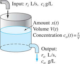
FIGURE 1.5.4.

The single-tank mixture problem.

The amount of solute that flows out of the tank during the same time interval depends on the concentration $c_{0} (t)$ $c_{0} (t)$ of solute in the solution at time t. But as noted in Fig. 1.5.4, $c_{0} (t) = x (t) / V (t)$ $c_{0} (t) = x (t) / V (t)$ , where V(t) denotes the volume (not constant unless $r_{i} = r_{0}$ $r_{i} = r_{0}$ ) of solution in the tank at time t. Then

Δ x = {grams input} - {grams output} \approx r_{i} c_{i} Δ t - r_{0} c_{0} Δ t .

$Δ x = {grams input} - {grams output} \approx r_{i} c_{i} Δ t - r_{0} c_{0} Δ t .$

We now divide by $Δ t$ $Δ t$ :

\frac{Δ x}{Δ t} \approx r_{i} c_{i} - r_{0} c_{0} .

$\frac{Δ x}{Δ t} \approx r_{i} c_{i} - r_{0} c_{0} .$

Finally, we take the limit as $Δ t \to 0$ $Δ t \to 0$ ; if all the functions involved are continuous and x(t) is differentiable, then the error in this approximation also approaches zero, and we obtain the differential equation

\frac{d x}{d t} \approx r_{i} c_{i} - r_{0} c_{0},

$\frac{d x}{d t} \approx r_{i} c_{i} - r_{0} c_{0},$ (16)

in which $r_{i}, c_{i}$ $r_{i}, c_{i}$ , and $r_{0}$ $r_{0}$ are constants, but $c_{0}$ $c_{0}$ denotes the variable concentration

c_{0} (t) = \frac{x (t)}{V (t)}

$c_{0} (t) = \frac{x (t)}{V (t)}$ (17)

of solute in the tank at time t. Thus the amount x(t) of solute in the tank satisfies the differential equation

\frac{d x}{d t} = r_{i} c_{i} - \frac{r_{0}}{V} x .

$\frac{d x}{d t} = r_{i} c_{i} - \frac{r_{0}}{V} x .$ (18)

If $V_{0} = V (0)$ $V_{0} = V (0)$ , then $V (t) = V_{0} + (r_{i} - r_{0}) t$ $V (t) = V_{0} + (r_{i} - r_{0}) t$ , so Eq. (18) is a linear first-order differential equation for the amount x(t) of solute in the tank at time t.

Important

Equation (18) need not be committed to memory. It is the process we used to obtain that equation—examination of the behavior of the system over a short time interval $[t, t + Δ t]$ $[t, t + Δ t]$ —that you should strive to understand, because it is a very useful tool for obtaining all sorts of differential equations.

Remark

It was convenient for us to use g/L mass/volume units in deriving Eq. (18). But any other consistent system of units can be used to measure amounts of solute and volumes of solution. In the following example we measure both in cubic kilometers.

Example 4

Mixture problem Assume that Lake Erie has a volume of ${480 km}^{3}$ ${480 km}^{3}$ and that its rate of inflow (from Lake Huron) and outflow (to Lake Ontario) are both ${350 km}^{3}$ ${350 km}^{3}$ per year. Suppose that at the time $t = 0$ $t = 0$ (years), the pollutant concentration of Lake Erie—caused by past industrial pollution that has now been ordered to cease—is five times that of Lake Huron. If the outflow henceforth is perfectly mixed lake water, how long will it take to reduce the pollution concentration in Lake Erie to twice that of Lake Huron?

Solution

Here we have

\begin{array}{rcl} V & = & 480 ({km}^{3}), \\ r_{i} & = & r_{0} = r = 350 ({km}^{3} / yr), \\ c_{i} & = & c (the pollutant concentration of Lake Huron), and \\ x_{0} & = & x (0) = 5 c V, \end{array}

$\begin{array}{rcl} V & = & 480 ({km}^{3}), \\ r_{i} & = & r_{0} = r = 350 ({km}^{3} / yr), \\ c_{i} & = & c (the pollutant concentration of Lake Huron), and \\ x_{0} & = & x (0) = 5 c V, \end{array}$

and the question is this: When is $x (t) = 2 c V$ $x (t) = 2 c V$ ? With this notation, Eq. (18) is the separable equation

\frac{d x}{d t} = r c - \frac{r}{V} x,

$\frac{d x}{d t} = r c - \frac{r}{V} x,$ (19)

which we rewrite in the linear first-order form

\frac{d x}{d t} + p x = q

$\frac{d x}{d t} + p x = q$ (20)

with constant coefficients $p = r / V, q = r c$ $p = r / V, q = r c$ , and integrating factor $ρ = e^{p t}$ $ρ = e^{p t}$ . You can either solve this equation directly or apply the formula in (12). The latter gives

\begin{array}{rcl} x (t) & = & e^{- p t} [x_{0} + \int_{0}^{t} q e^{p t} d t] = e^{- p t} [x_{0} + \frac{q}{p} (e^{p t} - 1)] \\ = & e^{- r t / V} [5 c V + \frac{r c}{r / V} (e^{r t / V} - 1)]; \\ x (t) & = & c V + 4 c V e^{- r t / V} . \end{array}

$\begin{array}{rcl} x (t) & = & e^{- p t} [x_{0} + \int_{0}^{t} q e^{p t} d t] = e^{- p t} [x_{0} + \frac{q}{p} (e^{p t} - 1)] \\ = & e^{- r t / V} [5 c V + \frac{r c}{r / V} (e^{r t / V} - 1)]; \\ x (t) & = & c V + 4 c V e^{- r t / V} . \end{array}$ (21)

To find when $x (t) = 2 c V$ $x (t) = 2 c V$ , we therefore need only solve the equation

\begin{array}{rcl} c V + 4 c V e^{- r t / V} = 2 c V & for & t = \frac{V}{r} \ln 4 = \frac{480}{350} \ln 4 \approx 1.901 (years) . \end{array}

$\begin{array}{rcl} c V + 4 c V e^{- r t / V} = 2 c V & for & t = \frac{V}{r} \ln 4 = \frac{480}{350} \ln 4 \approx 1.901 (years) . \end{array}$

Example 5

Mixture problem A 120-gallon (gal) tank initially contains 90 lb of salt dissolved in 90 gal of water. Brine containing 2 lb/gal of salt flows into the tank at the rate of 4 gal/min, and the well-stirred mixture flows out of the tank at the rate of 3 gal/min. How much salt does the tank contain when it is full?

Solution

The interesting feature of this example is that, due to the differing rates of inflow and outflow, the volume of brine in the tank increases steadily with $V (t) = 90 + t$ $V (t) = 90 + t$ gallons. The change $Δ x$ $Δ x$ in the amount x of salt in the tank from time t to time $t + Δ t$ $t + Δ t$ (minutes) is given by

Δ x \approx (4) (2) Δ t - 3 (\frac{x}{90 + t}) Δ t,

$Δ x \approx (4) (2) Δ t - 3 (\frac{x}{90 + t}) Δ t,$

so our differential equation is

\frac{d x}{d t} + \frac{3}{90 + t} x = 8 .

$\frac{d x}{d t} + \frac{3}{90 + t} x = 8 .$

An integrating factor is

ρ (x) = \exp (\int \frac{3}{90 + t} d t) = e^{3 \ln (90 + t)} = {(90 + t)}^{3},

$ρ (x) = \exp (\int \frac{3}{90 + t} d t) = e^{3 \ln (90 + t)} = {(90 + t)}^{3},$

which gives

\begin{array}{rcl} D_{t} [{(90 + t)}^{3} x] & = & 8 {(90 + t)}^{3}; \\ {(90 + t)}^{3} x & = & 2 {(90 + t)}^{4} + C . \end{array}

$\begin{array}{rcl} D_{t} [{(90 + t)}^{3} x] & = & 8 {(90 + t)}^{3}; \\ {(90 + t)}^{3} x & = & 2 {(90 + t)}^{4} + C . \end{array}$

Substitution of $x (0) = 90$ $x (0) = 90$ gives $C = - {(90)}^{4}$ $C = - {(90)}^{4}$ , so the amount of salt in the tank at time t is

x (t) = 2 (90 + t) - \frac{90^{4}}{{(90 + t)}^{3}} .

$x (t) = 2 (90 + t) - \frac{90^{4}}{{(90 + t)}^{3}} .$

The tank is full after 30 min, and when $t = 30$ $t = 30$ , we have

x (30) = 2 (90 + 30) - \frac{90^{4}}{120^{3}} \approx 202 (lb)

$x (30) = 2 (90 + 30) - \frac{90^{4}}{120^{3}} \approx 202 (lb)$

of salt in the tank.

1.5 Problems

Find general solutions of the differential equations in Problems 1 through 25. If an initial condition is given, find the corresponding particular solution. Throughout, primes denote derivatives with respect to x.

$y ′ + y = 2, y (0) = 0$ $y ′ + y = 2, y (0) = 0$
$y ′ - 2 y = 3 e^{2 x}, y (0) = 0$ $y ′ - 2 y = 3 e^{2 x}, y (0) = 0$
$y ′ + 3 y = 2 x e^{- 3 x}$ $y ′ + 3 y = 2 x e^{- 3 x}$
$y ′ - 2 x y = e^{x^{2}}$ $y ′ - 2 x y = e^{x^{2}}$
$x y ′ + 2 y = 3 x, y (1) = 5$ $x y ′ + 2 y = 3 x, y (1) = 5$
$x y ′ + 5 y = 7 x^{2}, y (2) = 5$ $x y ′ + 5 y = 7 x^{2}, y (2) = 5$
$2 x y ′ + y = 10 \sqrt{x}$ $2 x y ′ + y = 10 \sqrt{x}$
$3 x y ′ + y = 12 x$ $3 x y ′ + y = 12 x$
$x y ′ - y = x, y (1) = 7$ $x y ′ - y = x, y (1) = 7$
$2 x y ′ - 3 y = 9 x^{3}$ $2 x y ′ - 3 y = 9 x^{3}$
$x y ′ + y = 3 x y$ $x y ′ + y = 3 x y$ , $y (1) = 0$ $y (1) = 0$
$x y ′ + 3 y = 2 x^{5}$ $x y ′ + 3 y = 2 x^{5}$ , $y (2) = 1$ $y (2) = 1$
$y ′ + y = e^{x}$ $y ′ + y = e^{x}$ , $y (0) = 1$ $y (0) = 1$
$x y ′ - 3 y = x^{3}$ $x y ′ - 3 y = x^{3}$ , $y (1) = 10$ $y (1) = 10$
$y ′ + 2 x y = x$ $y ′ + 2 x y = x$ , $y (0) = - 2$ $y (0) = - 2$
$y ′ = (1 - y) \cos x$ $y ′ = (1 - y) \cos x$ , $y (π) = 2$ $y (π) = 2$
$(1 + x) y ′ + y = \cos x$ $(1 + x) y ′ + y = \cos x$ , $y (0) = 1$ $y (0) = 1$
$x y ′ = 2 y + x^{3} \cos x$ $x y ′ = 2 y + x^{3} \cos x$
$y ′ + y \cot x = \cos x$ $y ′ + y \cot x = \cos x$
$y ′ = 1 + x + y + x y$ $y ′ = 1 + x + y + x y$ , $y (0) = 0$ $y (0) = 0$
$x y ′ = 3 y + x^{4} \cos x, y (2 π) = 0$ $x y ′ = 3 y + x^{4} \cos x, y (2 π) = 0$
$y ′ = 2 x y + 3 x^{2} \exp (x^{2})$ $y ′ = 2 x y + 3 x^{2} \exp (x^{2})$ , $y (0) = 5$ $y (0) = 5$
$x y ′ + (2 x - 3) y = 4 x^{4}$ $x y ′ + (2 x - 3) y = 4 x^{4}$
$(x^{2} + 4) y ′ + 3 x y = x$ $(x^{2} + 4) y ′ + 3 x y = x$ , $y (0) = 1$ $y (0) = 1$
$(x^{2} + 1) \frac{d y}{d x} + 3 x^{3} y = 6 x \exp (- \frac{3}{2} x^{2}), y (0) = 1$ $(x^{2} + 1) \frac{d y}{d x} + 3 x^{3} y = 6 x \exp (- \frac{3}{2} x^{2}), y (0) = 1$

Solve the differential equations in Problems 26 through 28 by regarding y as the independent variable rather than x.

$(1 - 4 x y^{2}) \frac{d y}{d x} = y^{3}$ $(1 - 4 x y^{2}) \frac{d y}{d x} = y^{3}$
$(x + y e^{y}) \frac{d y}{d x} = 1$ $(x + y e^{y}) \frac{d y}{d x} = 1$
$(1 + 2 x y) \frac{d y}{d x} = 1 + y^{2}$ $(1 + 2 x y) \frac{d y}{d x} = 1 + y^{2}$
Express the general solution of $d y / d x = 1 + 2 x y$ $d y / d x = 1 + 2 x y$ in terms of the error function

$erf (x) = \frac{2}{\sqrt{π}} \int_{0}^{x} e^{- t^{2}} d t .$ $erf (x) = \frac{2}{\sqrt{π}} \int_{0}^{x} e^{- t^{2}} d t .$
Express the solution of the initial value problem

$\begin{array}{l} 2 x \frac{d y}{d x} = y + 2 x \cos x, & y (1) = 0 \end{array}$ $\begin{array}{l} 2 x \frac{d y}{d x} = y + 2 x \cos x, & y (1) = 0 \end{array}$

as an integral as in Example 3 of this section.

Problems 31 and 32 illustrate—for the special case of first-order linear equations-techniques that will be important when we study higher—order linear equations in Chapter 3.

(a) Show that

$y_{c} (x) = C e^{- \int P (x) d x}$ $y_{c} (x) = C e^{- \int P (x) d x}$

is a general solution of $d y / d x + P (x) y = 0$ $d y / d x + P (x) y = 0$ . (b) Show that

$y_{p} (x) = e^{- \int P (x) d x} [\int (Q (x) e^{\int P (x) d x}) d x]$ $y_{p} (x) = e^{- \int P (x) d x} [\int (Q (x) e^{\int P (x) d x}) d x]$

is a particular solution of $d y / d x + P (x) y = Q (x)$ $d y / d x + P (x) y = Q (x)$ . (c) Suppose that $y_{c} (x)$ $y_{c} (x)$ is any general solution of $d y / d x + P (x) y = 0$ $d y / d x + P (x) y = 0$ and that $y_{p} (x)$ $y_{p} (x)$ is any particular solution of $d y / d x + P (x) y = Q (x)$ $d y / d x + P (x) y = Q (x)$ . Show that $y (x) = y_{c} (x) + y_{p} (x)$ $y (x) = y_{c} (x) + y_{p} (x)$ is a general solution of $d y / d x + P (x) y = Q (x)$ $d y / d x + P (x) y = Q (x)$ .
(a) Find constants A and B such that $y_{p} (x) = A \sin x + B \cos x$ $y_{p} (x) = A \sin x + B \cos x$ is a solution of $d y / d x + y = 2 \sin x$ $d y / d x + y = 2 \sin x$ . (b) Use the result of part (a) and the method of Problem 31 to find the general solution of $d y / d x + y = 2 \sin x$ $d y / d x + y = 2 \sin x$ . (c) Solve the initial value problem $d y / d x + y = 2 \sin x, y (0) = 1$ $d y / d x + y = 2 \sin x, y (0) = 1$ .

Mixture Problems

Problems 33 through 37 illustrate the application of linear first-order differential equations to mixture problems.

A tank contains 1000 liters (L) of a solution consisting of 100 kg of salt dissolved in water. Pure water is pumped into the tank at the rate of 5 L/s, and the mixture—kept uniform by stirring—is pumped out at the same rate. How long will it be until only 10 kg of salt remains in the tank?
Consider a reservoir with a volume of 8 billion cubic feet ( ${ft}^{3}$ ${ft}^{3}$ ) and an initial pollutant concentration of 0.25%. There is a daily inflow of 500 million ${ft}^{3}$ ${ft}^{3}$ of water with a pollutant concentration of 0.05% and an equal daily outflow of the well-mixed water in the reservoir. How long will it take to reduce the pollutant concentration in the reservoir to 0.10%?
Rework Example 4 for the case of Lake Ontario, which empties into the St. Lawrence River and receives inflow from Lake Erie (via the Niagara River). The only differences are that this lake has a volume of ${1640 km}^{3}$ ${1640 km}^{3}$ and an inflow-outflow rate of ${410 km}^{3} /$ ${410 km}^{3} /$ year.
A tank initially contains 60 gal of pure water. Brine containing 1 lb of salt per gallon enters the tank at 2 gal/min, and the (perfectly mixed) solution leaves the tank at 3 gal/min; thus the tank is empty after exactly 1 h. (a) Find the amount of salt in the tank after t minutes. (b) What is the maximum amount of salt ever in the tank?
A 400-gal tank initially contains 100 gal of brine containing 50 lb of salt. Brine containing 1 lb of salt per gallon enters the tank at the rate of 5 gal/s, and the well-mixed brine in the tank flows out at the rate of 3 gal/s. How much salt will the tank contain when it is full of brine?
Two tanks Consider the cascade of two tanks shown in Fig. 1.5.5, with $V_{1} = 100 (gal)$ $V_{1} = 100 (gal)$ and $V_{2} = 200 (gal)$ $V_{2} = 200 (gal)$ the volumes of brine in the two tanks. Each tank also initially contains 50 lb of salt. The three flow rates indicated in the figure are each 5 gal/min, with pure water flowing into tank 1. (a) Find the amount x(t) of salt in tank 1 at time t.(b) Suppose that y(t) is the amount of salt in tank 2 at time t. Show first that

$\frac{d y}{d t} = \frac{5 x}{100} - \frac{5 y}{200},$ $\frac{d y}{d t} = \frac{5 x}{100} - \frac{5 y}{200},$

and then solve for y(t), using the function x(t) found in part (a).(c) Finally, find the maximum amount of salt ever in tank 2.

FIGURE 1.5.5.

A cascade of two tanks.
Two tanks Suppose that in the cascade shown in Fig. 1.5.5, tank 1 initially contains 100 gal of pure ethanol and tank 2 initially contains 100 gal of pure water. Pure water flows into tank 1 at 10 gal/min, and the other two flow rates are also 10 gal/min.(a) Find the amounts x(t) and y(t) of ethanol in the two tanks at time $t ≧ 0 .$ $t ≧ 0 .$ (b) Find the maximum amount of ethanol ever in tank 2.
Multiple tanks A multiple cascade is shown in Fig. 1.5.6. At time $t = 0$ $t = 0$ , tank 0 contains 1 gal of ethanol and 1 gal of water; all the remaining tanks contain 2 gal of pure water each. Pure water is pumped into tank 0 at 1 gal/min, and the varying mixture in each tank is pumped into the one below it at the same rate. Assume, as usual, that the mixtures are kept perfectly uniform by stirring. Let $x_{n} (t)$ $x_{n} (t)$ denote the amount of ethanol in tank n at time t.

FIGURE 1.5.6.

A multiple cascade.

(a) Show that $x_{0} (t) = e^{- t / 2}$ $x_{0} (t) = e^{- t / 2}$ . (b) Show by induction on n that

$x_{n} (t) = \frac{t^{n} e^{- t / 2}}{n! 2^{n}} for n \geq 0 .$ $x_{n} (t) = \frac{t^{n} e^{- t / 2}}{n! 2^{n}} for n \geq 0 .$

(c) Show that the maximum value of $x_{n} (t)$ $x_{n} (t)$ for $n > 0$ $n > 0$ is $M_{n} = x_{n} (2 n) = n^{n} e^{- n} / n!$ $M_{n} = x_{n} (2 n) = n^{n} e^{- n} / n!$ . (d) Conclude from Stirling’s approximation $n! \approx n^{n} e^{- n} \sqrt{2 π n}$ $n! \approx n^{n} e^{- n} \sqrt{2 π n}$ that $M_{n} \approx {(2 π n)}^{- 1/2}$ $M_{n} \approx {(2 π n)}^{- 1/2}$ .
Retirement savings A 30-year-old woman accepts an engineering position with a starting salary of $30,000 per year. Her salary S(t) increases exponentially, with $S (t) = 30 e^{t / 20}$ $S (t) = 30 e^{t / 20}$ thousand dollars after t years. Meanwhile, 12% of her salary is deposited continuously in a retirement account, which accumulates interest at a continuous annual rate of 6%.(a) Estimate $Δ A$ $Δ A$ in terms of $Δ t$ $Δ t$ to derive the differential equation satisfied by the amount A(t) in her retirement account after t years.(b) Compute $A (40)$ $A (40)$ , the amount available for her retirement at age 70.
Falling hailstone Suppose that a falling hailstone with density $δ = 1$ $δ = 1$ starts from rest with negligible radius $r = 0$ $r = 0$ . Thereafter its radius is $r = k t$ $r = k t$ (k is a constant) as it grows by accretion during its fall. Use Newton#x2019;s second law—according to which the net force F acting on a possibly variable mass m equals the time rate of change $d p / d t$ $d p / d t$ of its momentum $p = m v$ $p = m v$ —to set up and solve the initial value problem

$\begin{array}{l} \frac{d}{d t} (m v) = m g, & v (0) = 0, \end{array}$ $\begin{array}{l} \frac{d}{d t} (m v) = m g, & v (0) = 0, \end{array}$

where m is the variable mass of the hailstone, $v = d y / d t$ $v = d y / d t$ is its velocity, and the positive y-axis points downward. Then show that $d v / d t = g / 4$ $d v / d t = g / 4$ . Thus the hailstone falls as though it were under one-fourth the influence of gravity.
Figure 1.5.7 shows a slope field and typical solution curves for the equation $y ′ = x - y$ $y ′ = x - y$ . (a) Show that every solution curve approaches the straight line $y = x - 1$ $y = x - 1$ as $x \to + \infty$ $x \to + \infty$ . (b) For each of the five values $y_{1} = 3.998, 3.999, 4.000, 4.001$ $y_{1} = 3.998, 3.999, 4.000, 4.001$ , and 4.002, determine the initial value $y_{0}$ $y_{0}$ (accurate to four decimal places) such that $y (5) = y_{1}$ $y (5) = y_{1}$ for the solution satisfying the initial condition $y (- 5) = y_{0}$ $y (- 5) = y_{0}$ .

FIGURE 1.5.7.

Slope field and solution curves for $y^{′} = x - y .$ $y^{′} = x - y .$
Figure 1.5.8 shows a slope field and typical solution curves for the equation $y ′ = x + y$ $y ′ = x + y$ . (a) Show that every solution curve approaches the straight line $y = - x - 1$ $y = - x - 1$ as $x \to - \infty$ $x \to - \infty$ . (b) For each of the five values $y_{1} = - 10, - 5, 0, 5$ $y_{1} = - 10, - 5, 0, 5$ , and 10, determine the initial value $y_{0}$ $y_{0}$ (accurate to five decimal places) such that $y (5) = y_{1}$ $y (5) = y_{1}$ for the solution satisfying the initial condition $y (- 5) = y_{0}$ $y (- 5) = y_{0}$ .

FIGURE 1.5.8.

Slope field and solution curves for $y^{′} = x + y .$ $y^{′} = x + y .$

Polluted Reservoir

Problems 45 and 46 deal with a shallow reservoir that has a one-square-kilometer water surface and an average water depth of 2 meters. Initially it is filled with fresh water, but at time $t = 0$ $t = 0$ water contaminated with a liquid pollutant begins flowing into the reservoir at the rate of 200 thousand cubic meters per month. The well-mixed water in the reservoir flows out at the same rate. Your first task is to find the amount x(t) of pollutant (in millions of liters) in the reservoir after t months.

The incoming water has a pollutant concentration of $c (t) = 10$ $c (t) = 10$ liters per cubic meter ( ${L/m}^{3}$ ${L/m}^{3}$ ). Verify that the graph of x(t) resembles the steadily rising curve in Fig. 1.5.9, which approaches asymptotically the graph of the equilibrium solution $x (t) \equiv 20$ $x (t) \equiv 20$ that corresponds to the reservoir’s long-term pollutant content. How long does it take the pollutant concentration in the reservoir to reach $10 {L/m}^{3}$ $10 {L/m}^{3}$ ?
The incoming water has pollutant concentration $c (t) = 10 (1 + \cos t) {L/m}^{3}$ $c (t) = 10 (1 + \cos t) {L/m}^{3}$ that varies between 0 and 20, with an average concentration of $10 {L/m}^{3}$ $10 {L/m}^{3}$ and a period of oscillation of slightly over $6 \frac{1}{4}$ $6 \frac{1}{4}$ months. Does it seem predictable that the lake’s pollutant content should ultimately oscillate periodically about an average level of 20 million liters? Verify that the graph of x(t) does, indeed, resemble the oscillatory curve shown in Fig. 1.5.9. How long does it take the pollutant concentration in the reservoir to reach $10 {L/m}^{3}$ $10 {L/m}^{3}$ ?

FIGURE 1.5.9.

Graphs of solutions in Problems 45 and 46.

1.5 Application Indoor Temperature Oscillations

For an interesting applied problem that involves the solution of a linear differential equation, consider indoor temperature oscillations that are driven by outdoor temperature oscillations of the form

A (t) = a_{0} + a_{1} \cos ω t + b_{1} \sin ω t .

$A (t) = a_{0} + a_{1} \cos ω t + b_{1} \sin ω t .$ (1)

If $ω = π / 12$ $ω = π / 12$ , then these oscillations have a period of 24 hours (so that the cycle of outdoor temperatures repeats itself daily) and Eq. (1) provides a realistic model for the temperature outside a house on a day when no change in the overall day-to-day weather pattern is occurring. For instance, for a typical July day in Athens, Georgia with a minimum temperature of $70 ° F$ $70 ° F$ when $t = 4$ $t = 4$ (4 a.m.) and a maximum of $90 ° F$ $90 ° F$ when $t = 16$ $t = 16$ (4 p.m.), we would take

A (t) = 80 - 10 \cos ω t (t - 4) = 80 - 5 \cos ω t - 5 \sqrt{3} \sin ω t .

$A (t) = 80 - 10 \cos ω t (t - 4) = 80 - 5 \cos ω t - 5 \sqrt{3} \sin ω t .$ (2)

We derived Eq. (2) by using the identity $\cos (α - β) = \cos α \cos β + \sin α \sin β$ $\cos (α - β) = \cos α \cos β + \sin α \sin β$ to get $a_{0} = 80, a_{1} = - 5$ $a_{0} = 80, a_{1} = - 5$ , and $b_{1} = - 5 \sqrt{3}$ $b_{1} = - 5 \sqrt{3}$ in Eq. (1).

If we write Newton’s law of cooling (Eq. (3) of Section 1.1) for the corresponding indoor temperature u(t) at time t, but with the outside temperature A(t) given by Eq. (1) instead of a constant ambient temperature A, we get the linear first-order differential equation

\frac{d u}{d t} = - k (u - A (t));

$\frac{d u}{d t} = - k (u - A (t));$

that is,

\frac{d u}{d t} + k u = k (a_{0} + a_{1} \cos ω t + b_{1} \sin ω t)

$\frac{d u}{d t} + k u = k (a_{0} + a_{1} \cos ω t + b_{1} \sin ω t)$ (3)

with coefficient functions $P (t) \equiv k$ $P (t) \equiv k$ and $Q (t) = k A (t)$ $Q (t) = k A (t)$ . Typical values of the proportionality constant k range from 0.2 to 0.5 (although k might be greater than 0.5 for a poorly insulated building with open windows, or less than 0.2 for a well-insulated building with tightly sealed windows).

Scenario: Suppose that our air conditioner fails at time $t_{0} = 0$ $t_{0} = 0$ one midnight, and we cannot afford to have it repaired until payday at the end of the month. We therefore want to investigate the resulting indoor temperatures that we must endure for the next several days.

Begin your investigation by solving Eq. (3) with the initial condition $u (0) = u_{0}$ $u (0) = u_{0}$ (the indoor temperature at the time of the failure of the air conditioner). You may want to use the integral formulas in 49 and 50 of the endpapers, or possibly a computer algebra system. You should get the solution

u (t) = a_{0} + c_{0} e^{- k t} + c_{1} \cos ω t + d_{1} \sin ω t,

$u (t) = a_{0} + c_{0} e^{- k t} + c_{1} \cos ω t + d_{1} \sin ω t,$ (4)

where

\begin{array}{rcl} c_{0} & = & u_{0} - a_{0} - \frac{k^{2} a_{1} - k ω b_{1}}{k^{2} + ω^{2}}, \\ c_{1} & = & \frac{k^{2} a_{1} - k ω b_{1}}{k^{2} + ω^{2}}, d_{1} = \frac{k ω a_{1} + k^{2} b_{1}}{k^{2} + ω^{2}} \end{array}

$\begin{array}{rcl} c_{0} & = & u_{0} - a_{0} - \frac{k^{2} a_{1} - k ω b_{1}}{k^{2} + ω^{2}}, \\ c_{1} & = & \frac{k^{2} a_{1} - k ω b_{1}}{k^{2} + ω^{2}}, d_{1} = \frac{k ω a_{1} + k^{2} b_{1}}{k^{2} + ω^{2}} \end{array}$

with $ω = π / 12$ $ω = π / 12$ .

With $a_{0} = 80, a_{1} = - 5, b_{1} = - 5 \sqrt{3}$ $a_{0} = 80, a_{1} = - 5, b_{1} = - 5 \sqrt{3}$ (as in Eq. (2)), $ω = π / 12$ $ω = π / 12$ , and $k = 0.2$ $k = 0.2$ (for instance), this solution reduces (approximately) to

u (t) = 80 + e^{- t / 5} (u_{0} - 82.3351) + (2.3351) \cos \frac{π t}{12} - (5.6036) \sin \frac{π t}{12} .

$u (t) = 80 + e^{- t / 5} (u_{0} - 82.3351) + (2.3351) \cos \frac{π t}{12} - (5.6036) \sin \frac{π t}{12} .$ (5)

Observe first that the “damped” exponential term in Eq. (5) approaches zero as $t \to + \infty$ $t \to + \infty$ , leaving the long-term “steady periodic” solution

u_{sp} (t) = 80 + (2.3351) \cos \frac{π t}{12} - (5.6036) \sin \frac{π t}{12} .

$u_{sp} (t) = 80 + (2.3351) \cos \frac{π t}{12} - (5.6036) \sin \frac{π t}{12} .$ (6)

Consequently, the long-term indoor temperatures oscillate every 24 hours around the same average temperature $80 ° F$ $80 ° F$ as the average outdoor temperature.

Figure 1.5.10 shows a number of solution curves corresponding to possible initial temperatures $u_{0}$ $u_{0}$ ranging from $65 ° F$ $65 ° F$ to $95 ° F$ $95 ° F$ . Observe that—whatever the initial temperature—the indoor temperature “settles down” within about 18 hours to a periodic daily oscillation. But the amplitude of temperature variation is less indoors than outdoors. Indeed, using the trigonometric identity mentioned earlier, Eq. (6) can be rewritten (verify this!) as

FIGURE 1.5.10.

Solution curves given by Eq. (5) with $u_{0} = 65, 68, 71, \dots, 92, 95$ $u_{0} = 65, 68, 71, \dots, 92, 95$ .

\begin{array}{rcl} u (t) & = & 80 - (6.0707) \cos (\frac{π t}{12} - 1.9656) \\ = & 80 - (6.0707) \cos \frac{π}{2} (t - 7.5082) . \end{array}

$\begin{array}{rcl} u (t) & = & 80 - (6.0707) \cos (\frac{π t}{12} - 1.9656) \\ = & 80 - (6.0707) \cos \frac{π}{2} (t - 7.5082) . \end{array}$ (7)

Do you see that this implies that the indoor temperature varies between a minimum of about $74 ° F$ $74 ° F$ and a maximum of about $86 ° F$ $86 ° F$ ?

Finally, comparison of Eqs. (2) and (7) indicates that the indoor temperature lags behind the outdoor temperature by about $7.5082 - 4 \approx 3.5$ $7.5082 - 4 \approx 3.5$ hours, as illustrated in Fig. 1.5.11. Thus the temperature inside the house continues to rise until about 7:30 p.m. each evening, so the hottest part of the day inside is early evening rather than late afternoon (as outside).

FIGURE 1.5.11.

Comparison of indoor and outdoor temperature oscillations.

For a personal problem to investigate, carry out a similar analysis using average July daily maximum/minimum figures for your own locale and a value of k appropriate to your own home. You might also consider a winter day instead of a summer day. (What is the winter-summer difference for the indoor temperature problem?) You may wish to explore the use of available technology both to solve the differential equation and to graph its solution for the indoor temperature in comparison with the outdoor temperature.

..................Content has been hidden....................

You can't read the all page of ebook, please click here login for view all page.

Table of Contents for 1.5 Linear First-Order Equations

Create new playlist

Sign In

Sign Up

Table of Contents for
1.5 Linear First-Order Equations