
1.3 Slope Fields and Solution Curves
Consider a differential equation of the form
![]()
where the right-hand function f(x,y)
Slope Fields and Graphical Solutions
There is a simple geometric way to think about solutions of a given differential equation y′=f(x,y)

FIGURE 1.3.1.
A solution curve for the differential equation y′=x−y
slope m1=x1−y1
m1=x1−y1 at the point (x1, y1)(x1, y1) ;slope m2=x2−y2
m2=x2−y2 at the point (x2, y2)(x2, y2) ; andslope m3=x3−y3
m3=x3−y3 at the point (x3, y3)(x3, y3) .
This geometric viewpoint suggests a graphical method for constructing approximate solutions of the differential equation y′=f(x,y)
Example 1
Figures 1.3.2 (a)–(d) show slope fields and solution curves for the differential equation
with the values k=2, 0.5, −1
A slope field suggests visually the general shapes of solution curves of the differential equation. Through each point a solution curve should proceed in such a direction that its tangent line is nearly parallel to the nearby line segments of the slope field. Starting at any initial point (a, b), we can attempt to sketch freehand an approximate solution curve that threads its way through the slope field, following the visible line segments as closely as possible.

FIGURE 1.3.2(a)
Slope field and solution curves for y′=2y

FIGURE 1.3.2(b)
Slope field and solution curves for y′=(0.5)y

FIGURE 1.3.2(c)
Slope field and solution curves for y′=−y

FIGURE 1.3.2(d)
Slope field and solution curves for y′=−3y
| x/y | −4 |
−3 |
−2 |
−1 |
0 | 1 | 2 | 3 | 4 |
| −4 |
0 | −1 |
−2 |
−3 |
−4 |
−5 |
−6 |
−7 |
−8 |
| −3 |
1 | 0 | −1 |
−2 |
−3 |
−4 |
−5 |
−6 |
−7 |
| −2 |
2 | 1 | 0 | −1 |
−2 |
−3 |
−4 |
−5 |
−6 |
| −1 |
3 | 2 | 1 | 0 | −1 |
−2 |
−3 |
−4 |
−5 |
| 0 | 4 | 3 | 2 | 1 | 0 | −1 |
−2 |
−3 |
−4 |
| 1 | 5 | 4 | 3 | 2 | 1 | 0 | −1 |
−2 |
−3 |
| 2 | 6 | 5 | 4 | 3 | 2 | 1 | 0 | −1 |
−2 |
| 3 | 7 | 6 | 5 | 4 | 3 | 2 | 1 | 0 | −1 |
| 4 | 8 | 7 | 6 | 5 | 4 | 3 | 2 | 1 | 0 |
FIGURE 1.3.3.
Values of the slope y′=x−y
Example 2
Construct a slope field for the differential equation y′=x−y
Solution
Figure 1.3.3 shows a table of slopes for the given equation. The numerical slope m=x−y
Although a spreadsheet program (for instance) readily constructs a table of slopes as in Fig. 1.3.3, it can be quite tedious to plot by hand a sufficient number of slope segments as in Fig. 1.3.4. However, most computer algebra systems include commands for quick and ready construction of slope fields with as many line segments as desired; such commands are illustrated in the application material for this section. The more line segments are constructed, the more accurately solution curves can be visualized and sketched. Figure 1.3.6 shows a “finer” slope field for the differential equation y′=x−y

FIGURE 1.3.4.
Slope field for y′=x−y

FIGURE 1.3.5.
The solution curve through (−4, 4).
If you look closely at Fig. 1.3.6, you may spot a solution curve that appears to be a straight line! Indeed, you can verify that the linear function y=x−1

FIGURE 1.3.6.
Slope field and typical solution curves for y′=x−y
Applications of Slope Fields
The next two examples illustrate the use of slope fields to glean useful information in physical situations that are modeled by differential equations. Example 3 is based on the fact that a baseball moving through the air at a moderate speed v (less than about 300 ft/s) encounters air resistance that is approximately proportional to v. If the baseball is thrown straight downward from the top of a tall building or from a hovering helicopter, then it experiences both the downward acceleration of gravity and an upward acceleration of air resistance. If the y-axis is directed downward, then the ball’s velocity v=dy/dt
A typical value of the air resistance proportionality constant might be k=0.16
Example 3
Falling baseball Suppose you throw a baseball straight downward from a helicopter hovering at an altitude of 3000 feet. You wonder whether someone standing on the ground below could conceivably catch it. In order to estimate the speed with which the ball will land, you can use your laptop’s computer algebra system to construct a slope field for the differential equation

FIGURE 1.3.7.
Slope field and typical solution curves for v′=32−0.16v
The result is shown in Fig. 1.3.7, together with a number of solution curves corresponding to different values of the initial velocity v(0) with which you might throw the baseball downward. Note that all these solution curves appear to approach the horizontal line v=200
Perhaps a catcher accustomed to 100 mi/h fastballs would have some chance of fielding this speeding ball.
Comment
If the ball’s initial velocity is v(0)=200
In Section 2.1 we will discuss in detail the logistic differential equation
that often is used to model a population P(t) that inhabits an environment with carrying capacity M. This means that M is the maximum population that this environment can sustain on a long-term basis (in terms of the maximum available food, for instance).
Example 4
Limiting population If we take k=0.0004

FIGURE 1.3.8.
Slope field and typical solution curves for P′=0.06P−0.0004P2
The positive term 0.06P on the right in (6) corresponds to natural growth at a 6%annual rate (with time t measured in years). The negative term −0.0004P2
Figure 1.3.8 shows a slope field for Eq. (6), together with a number of solution curves corresponding to possible different values of the initial population P(0). Note that all these solution curves appear to approach the horizontal line P=150
Comment
If the initial population is P(0)=150
so the population experiences no initial (instantaneous) change. It therefore remains unchanged, and hence P(t)≡150
Existence and Uniqueness of Solutions
Before one spends much time attempting to solve a given differential equation, it is wise to know that solutions actually exist. We may also want to know whether there is only one solution of the equation satisfying a given initial condition—that is, whether its solutions are unique.
Example 5
Failure of existence The initial value problem
y′=1x,y(0)=0(7)y'=1x,y(0)=0 has no solution, because no solution y(x)=∫(1/x)dx=ln |x|+C
y(x)=∫(1/x)dx=ln |x|+C of the differential equation is defined at x=0x=0 . We see this graphically in Fig. 1.3.9, which shows a direction field and some typical solution curves for the equation y′=1/xy'=1/x . It is apparent that the indicated direction field “forces” all solution curves near the y-axis to plunge downward so that none can pass through the point (0, 0).
FIGURE 1.3.9.
Direction field and typical solution curves for the equation y′=1/x.
y'=1/x. 
FIGURE 1.3.10.
Direction field and two different solution curves for the initial value problem y′=2√y, y(0)=0.
y'=2y√, y(0)=0. Failure of uniqueness On the other hand, you can readily verify that the initial value problem
y′=2√y,y(0)=0(8)y'=2y√,y(0)=0 has the two different solutions y1(x)=x2
y1(x)=x2 and y2(x)≡0y2(x)≡0 (see Problem 27). Figure 1.3.10 shows a direction field and these two different solution curves for the initial value problem in (8). We see that the curve y1(x)=x2y1(x)=x2 threads its way through the indicated direction field, whereas the differential equation y′=2√yy'=2y√ specifies slope y′=0y'=0 along the x-axis y2(x)=0y2(x)=0 .
Example 5 illustrates the fact that, before we can speak of “the” solution of an initial value problem, we need to know that it has one and only one solution. Questions of existence and uniqueness of solutions also bear on the process of mathematical modeling. Suppose that we are studying a physical system whose behavior is completely determined by certain initial conditions, but that our proposed mathematical model involves a differential equation not having a unique solution satisfying those conditions. This raises an immediate question as to whether the mathematical model adequately represents the physical system.
The theorem stated below implies that the initial value problem y′=f(x,y), y(a)=b

FIGURE 1.3.11.
The rectangle R and x-interval I of Theorem 1, and the solution curve y=y(x)
Remark 1
In the case of the differential equation dy/dx=−y
Remark 2
In the case of the differential equation dy/dx=2√y
Remark 3
In Example 7 of Section 1.1 we examined the especially simple differential equation dy/dx=y2
![]()
on some open x-interval containing a=0
that we discussed in Example 7. But y(x)=1/(1−x)

FIGURE 1.3.12.
The solution curve through the initial point (0, 1) leaves the rectangle R before it reaches the right side of R.
The following example shows that, if the function f(x,y)
Example 6
Consider the first-order differential equation
Applying Theorem 1 with f(x,y)=2y/x
satisfies Eq. (11) for any value of the constant C and for all values of the variable x. In particular, the initial value problem

FIGURE 1.3.13.
There are infinitely many solution curves through the point (0, 0), but no solution curves through the point (0, b) if b≠0
has infinitely many different solutions, whose solution curves are the parabolas y=Cx2
Observe that all these parabolas pass through the origin (0, 0), but none of them passes through any other point on the y-axis. It follows that the initial value problem in (13) has infinitely many solutions, but the initial value problem
has no solution if b≠0
Finally, note that through any point off the y-axis there passes only one of the parabolas y=Cx2
has a unique solution on any interval that contains the point x=a
a unique solution near (a, b) if a≠0
a≠0 ;no solution if a=0
a=0 but b≠0b≠0 ;infinitely many solutions if a=b=0
a=b=0 .
Still more can be said about the initial value problem in (15). Consider a typical initial point off the y-axis—for instance the point (−1,1)
is continuous and satisfies the initial value problem

FIGURE 1.3.14.
There are infinitely many solution curves through the point (1, −1).
For a particular value of C, the solution curve defined by (16) consists of the left half of the parabola y=x2
We therefore see that Theorem 1 (if its hypotheses are satisfied) guarantees uniqueness of the solution near the initial point (a, b), but a solution curve through (a, b) may eventually branch elsewhere so that uniqueness is lost. Thus a solution may exist on a larger interval than one on which the solution is unique. For instance, the solution y(x)=x2
1.3 Problems
In Problems 1 through 10, we have provided the slope field of the indicated differential equation, together with one or more solution curves. Sketch likely solution curves through the additional points marked in each slope field.
dydx=−y−sin x
dydx=−y−sin x 
FIGURE 1.3.15.
dydx=x+y
dydx=x+y 
FIGURE 1.3.16.
dydx=y−sin x
dydx=y−sin x 
FIGURE 1.3.17.
dydx=x−y
dydx=x−y 
FIGURE 1.3.18.
dydx=y−x+1
dydx=y−x+1 
FIGURE 1.3.19.
dydx=x−y+1
dydx=x−y+1 
FIGURE 1.3.20.
dydx=sin x+sin y
dydx=sin x+sin y 
FIGURE 1.3.21.
dydx=x2−y
dydx=x2−y 
FIGURE 1.3.22.
dydx=x2−y−2
dydx=x2−y−2 
FIGURE 1.3.23.
dydx=−x2+sin y
dydx=−x2+sin y 
FIGURE 1.3.24.
A more detailed version of Theorem 1 says that, if the function f(x,y)
dydx=2x2y2;y(1)=−1
dydx=2x2y2;y(1)=−1 dydx=x ln y;y(1)=1
dydx=x ln y;y(1)=1 dydx=3√y;y(0)=1
dydx=y√3;y(0)=1 dydx=3√y;y(0)=0
dydx=y√3;y(0)=0 dydx=√x−y;y(2)=2
dydx=x−y−−−−−√;y(2)=2 dydx=√x−y;y(2)=1
dydx=x−y−−−−−√;y(2)=1 ydydx=x−1;y(0)=1
ydydx=x−1;y(0)=1 ydydx=x−1;y(1)=0
ydydx=x−1;y(1)=0 dydx=ln (1+y2);y(0)=0
dydx=ln (1+y2);y(0)=0 dydx=x2−y2;y(0)=1
dydx=x2−y2;y(0)=1
In Problems 21 and 22, first use the method of Example 2 to construct a slope field for the given differential equation. Then sketch the solution curve corresponding to the given initial condition. Finally, use this solution curve to estimate the desired value of the solution y(x).
y′=x+y
y'=x+y , y(0)=0y(0)=0 ; y(−4)=y(−4)= ?y′=y−x
y'=y−x , y(4)=0y(4)=0 ; y(−4)=y(−4)= ?
Problems 23 and 24 are like Problems 21 and 22, but now use a computer algebra system to plot and print out a slope field for the given differential equation. If you wish (and know how), you can check your manually sketched solution curve by plotting it with the computer.
y′=x2+y2−1
y'=x2+y2−1 , y(0)=0y(0)=0 ; y(2)=y(2)= ?y′=x+12y2
y'=x+12y2 , y(−2)=0y(−2)=0 ; y(2)=y(2)= ?Falling Parachutist You bail out of the helicopter of Example 3 and pull the ripcord of your parachute. Now k=1.6
k=1.6 in Eq. (3), so your downward velocity satisfies the initial value problemdvdt=32−1.6v,v(0)=0.dvdt=32−1.6v,v(0)=0. In order to investigate your chances of survival, construct a slope field for this differential equation and sketch the appropriate solution curve. What will your limiting velocity be? Will a strategically located haystack do any good? How long will it take you to reach 95% of your limiting velocity?
Deer Population Suppose the deer population P(t) in a small forest satisfies the logistic equation
dPdt=0.0225P−0.0003P2.dPdt=0.0225P−0.0003P2. Construct a slope field and appropriate solution curve to answer the following questions: If there are 25 deer at time t=0
t=0 and t is measured in months, how long will it take the number of deer to double? What will be the limiting deer population?
The next seven problems illustrate the fact that, if the hypotheses of Theorem 1 are not satisfied, then the initial value problem y′=f(x,y), y(a)=b
Verify that if c is a constant, then the function defined piecewise by
y(x)={0for x≦c,(x−c)2for x>cy(x)={0(x−c)2for x≦c,for x>c satisfies the differential equation y′=2√y
y'=2y√ for all x (including the point x=cx=c ). Construct a figure illustrating the fact that the initial value problem y′=2√y, y(0)=0y'=2y√, y(0)=0 has infinitely many different solutions.For what values of b does the initial value problem y′=2√y, y(0)=b
y'=2y√, y(0)=b have (i) no solution, (ii) a unique solution that is defined for all x?
Verify that if k is a constant, then the function y(x)≡kx
y(x)≡kx satisfies the differential equation xy′=yxy'=y for all x. Construct a slope field and several of these straight line solution curves. Then determine (in terms of a and b) how many different solutions the initial value problem xy′=y, y(a)=bxy'=y, y(a)=b has—one, none, or infinitely many.Verify that if c is a constant, then the function defined piecewise by
y(x)={0for x≦c,(x−c)3for x>cy(x)={0(x−c)3for x≦c,for x>c satisfies the differential equation y′=3y2/3
y'=3y2/3 for all x. Can you also use the “left half” of the cubic y=(x−c)3y=(x−c)3 in piecing together a solution curve of the differential equation? (See Fig. 1.3.25.) Sketch a variety of such solution curves. Is there a point (a, b) of the xy-plane such that the initial value problem y′=3y2/3, y(a)=by'=3y2/3, y(a)=b has either no solution or a unique solution that is defined for all x? Reconcile your answer with Theorem 1.
FIGURE 1.3.25.
A suggestion for Problem 29.
Verify that if c is a constant, then the function defined piecewise by
y(x)={+1if x≦c,cos(x−c)if c<x<c+π,−1if x≧c+πsatisfies the differential equation y′=−√1−y2 for all x. (Perhaps a preliminary sketch with c=0 will be helpful.) Sketch a variety of such solution curves. Then determine (in terms of a and b) how many different solutions the initial value problem y′=−√1−y2, y(a)=b has.
Carry out an investigation similar to that in Problem 30, except with the differential equation y′=+√1−y2. Does it suffice simply to replace cos(x−c) with sin(x−c) in piecing together a solution that is defined for all x?
Verify that if c>0, then the function defined piecewise by
y(x)={0if x2≦c,(x2−c)2if x2>csatisfies the differential equation y′=4x√y for all x. Sketch a variety of such solution curves for different values of c. Then determine (in terms of a and b) how many different solutions the initial value problem y′=4x√y, y(a)=b has.
If c≠0, verify that the function defined by y(x)=x/(cx−1) (with the graph illustrated in Fig. 1.3.26) satisfies the differential equation x2y′+y2=0 if x≠1/c. Sketch a variety of such solution curves for different values of c. Also, note the constant-valued function y(x)≡0 that does not result from any choice of the constant c. Finally, determine (in terms of a and b) how many different solutions the initial value problem x2y′+y2=0, y(a)=b has.

FIGURE 1.3.26.
Slope field for x2y′+y2=0 and graph of a solution y(x)=x/(cx−1).
Use the direction field of Problem 5 to estimate the values at x=1 of the two solutions of the differential equation y′=y−x+1 with initial values y(−1)=−1.2 and y(−1)=−0.8.
Use a computer algebra system to estimate the values at x=3 of the two solutions of this differential equation with initial values y(−3)=−3.01 and y(−3)=−2.99.
The lesson of this problem is that small changes in initial conditions can make big differences in results.
Use the direction field of Problem 6 to estimate the values at x=2 of the two solutions of the differential equation y′=x−y+1 with initial values y(−3)=−0.2 and y(−3)=+0.2.
Use a computer algebra system to estimate the values at x=2 of the two solutions of this differential equation with initial values y(−3)=−0.5 and y(−3)=+0.5.
The lesson of this problem is that big changes in initial conditions may make only small differences in results.
1.3 Application Computer-Generated Slope Fields and Solution Curves
Widely available computer algebra systems and technical computing environments include facilities to automate the construction of slope fields and solution curves, as do some graphing calculators (see Figs. 1.3.27–29).
The Expanded Applications site at the URL indicated in the margin includes a discussion of Maple™, Mathematica™, and Matlab™ resources for the investigation of differential equations. For instance, the Maple command
with(DEtools):
DEplot(diff(y(x),x)=sin(x-y(x)), y(x), x=-5..5, y=-5..5);
and the Mathematica command
VectorPlot[{1, Sin[x-y]},{x, -5, 5}, {y, -5, 5}]produce slope fields similar to the one shown in Fig. 1.3.29. Figure 1.3.29 itself was generated with the Matlab program dfield [John Polking and David Arnold, Ordinary Differential Equations Using Matlab, 3rd edition, Hoboken, NJ: Pearson, 2003] that is freely available for educational use (math.rice.edu/~dfield). This web site also provides a stand-alone Java version of that can be used in a web browser. When a differential equation is entered in the dfield setup menu (Fig. 1.3.30), you can (with mouse button clicks) plot both a slope field and the solution curve (or curves) through any desired point (or points). Another freely available and user-friendly Matlab-based ODE package with impressive graphical capabilities is Iode (www.math.uiuc.edu/iode).

FIGURE 1.3.27.
TI-84 Plus CE™ graphing calculator and TI-Nspire™ CX CAS handheld. Screenshot from Texas Instruments Incorporated. Courtesy of Texas Instruments Incorporated.
Modern technology platforms offer even further interactivity by allowing the user to vary initial conditions and other parameters “in real time.” Mathematica’s Manipulate command was used to generate Fig. 1.3.31, which shows three particular solutions of the differential equation dy/dx=sin(x−y). The solid curve corresponds to the initial condition y(1)=0. As the “locator point” initially at (1, 0) is dragged—by mouse or touchpad—to the point (0, 3) or (2,−2), the solution curve immediately follows, resulting in the dashed curves shown. The TI-Nspire CX CAS has similar capability; indeed, as Fig. 1.3.28 appears on the Nspire display, each of the initial points (0,b) can be dragged to different locations using the Nspire’s touchpad, with the corresponding solution curves being instantly redrawn.
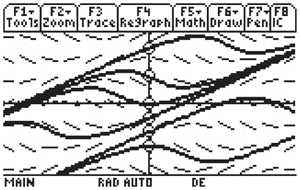
FIGURE 1.3.28.
Slope field and solution curves for the differential equation
with initial points (0, b), b=−3, −1, −2, 0, 2, 4 and window −5≦x, y≦5 on a TI-89 graphing calculator.

FIGURE 1.3.29.
Computer-generated slope field and solution curves for the differential equation y′=sin(x−y).

FIGURE 1.3.30.
Matlab dfield setup to construct slope field and solution curves for y′=sin(x−y).

FIGURE 1.3.31.
Interactive Mathematica solution of the differential equation y′=sin(x−y). The “locator point” corresponding to the initial condition y(1)=0 can be dragged to any other point in the display, causing the solution curve to be automatically redrawn.
Use a graphing calculator or computer system in the following investigations. You might warm up by generating the slope fields and some solution curves for Problems 1 through 10 in this section.
Investigation A: Plot a slope field and typical solution curves for the differential equation dy/dx=sin(x−y), but with a larger window than that of Fig. 1.3.29. With −10≦x≦10, −10≦y≦10, for instance, a number of apparent straight line solution curves should be visible, especially if your display allows you to drag the initial point interactively from upper left to lower right.
Substitute y=ax+b in the differential equation to determine what the coefficients a and b must be in order to get a solution. Are the results consistent with what you see on the display?
A computer algebra system gives the general solution
y(x)=x−2 tan−1(x−2−Cx−C).Plot this solution with selected values of the constant C to compare the resulting solution curves with those indicated in Fig. 1.3.28. Can you see that no value of C yields the linear solution y=x−π/2 corresponding to the initial condition y(π/2)=0? Are there any values of C for which the corresponding solution curves lie close to this straight line solution curve?
Investigation B: For your own personal investigation, let n be the smallest digit in your student ID number that is greater than 1, and consider the differential equation
First investigate (as in part (a) of Investigation A) the possibility of straight line solutions.
Then generate a slope field for this differential equation, with the viewing window chosen so that you can picture some of these straight lines, plus a sufficient number of nonlinear solution curves that you can formulate a conjecture about what happens to y(x) as x→+∞. State your inference as plainly as you can. Given the initial value y(0)=y0, try to predict (perhaps in terms of y0) how y(x) behaves as x→+∞.
A computer algebra system gives the general solution
y(x)=1n[x+2 tan−1(1x−C)].Can you make a connection between this symbolic solution and your graphically generated solution curves (straight lines or otherwise)?