Search in book...
Toggle Font Controls
Create new playlist

Name your new playlist

Playlist description (optional)
Sign In

Email address

Password

Forgot Password?

or

Continue with Facebook

Continue with Google
Sign Up

Full Name

Email address

Confirm Email Address

Password

or

Continue with Facebook

Continue with Google

7.6 Multiple Eigenvalue Solutions

In Section 7.3 we saw that if the n×n $n \times n$ matrix A has n distinct (real or complex) eigenvalues $λ_{1}, λ_{2}, \dots, λ_{n}$ with respective associated eigenvectors $v_{1}, v_{2}, \dots, v_{n}$ , then a general solution of the system

$\frac{d x}{d t} = A x$ (1)

is given by

$x (t) = c_{1} v_{1} e^{λ_{1} t} + c_{2} v_{2} e^{λ_{2} t} + \dots + c_{n} v_{n} e^{λ_{n} t}$ (2)

with arbitrary constants $c_{1}, c_{2}, \dots, c_{n}$ . In this section we discuss the situation when the characteristic equation

$| A - λ I | = 0$ (3)

does not have n distinct roots, and thus has at least one repeated root.

An eigenvalue is of multiplicity k if it is a k-fold root of Eq. (3). For each eigenvalue $λ$ , the eigenvector equation

$| A - λ I | v = 0$ (4)

has at least one nonzero solution v, so there is at least one eigenvector associated with $λ$ . But an eigenvalue of multiplicity $k > 1$ may have fewer than k linearly independent associated eigenvectors. In this case we are unable to find a “complete set” of n linearly independent eigenvectors of A, as needed to form the general solution in (2).

Let us call an eigenvalue of multiplicity k complete if it has k linearly independent associated eigenvectors. If every eigenvalue of the matrix A is complete, then—because eigenvectors associated with different eigenvalues are linearly independent—it follows that A does have a complete set of n linearly independent eigenvectors $v_{1}, v_{2}, \dots, v_{n}$ associated with the eigenvalues $λ_{1}, λ_{2}, \dots, λ_{n}$ (each repeated with its multiplicity). In this case a general solution of $x ′ = A x$ is still given by the usual combination in (2).

Example 1

Find a general solution of the system

$x^{′} = [\begin{array}{r} 9 & 4 & 0 \\ - 6 & - 1 & 0 \\ 6 & 4 & 3 \end{array}] x .$ (5)

Solution

The characteristic equation of the coefficient matrix A in Eq. (5) is

$\begin{aligned} | A - λ I | & = & | \begin{array}{c} 9 - λ & 4 & 0 \\ - 6 & - 1 - λ & 0 \\ 6 & 4 & 3 - λ \end{array} | \\ = & (3 - λ) [(9 - λ) (- 1 - λ) + 24] \\ = & (3 - λ) (15 - 8 λ + λ^{2}) \\ = & (5 - λ) {(3 - λ)}^{2} = 0. \end{aligned}$

Thus A has the distinct eigenvalue $λ_{1} = 5$ and the repeated eigenvalue $λ_{2} = 3$ of multiplicity $k = 2$ .

Case 1: $λ_{1} = 5$ . The eigenvector equation $(A - λ I) v = 0$ , where $v = {[a b c]}^{T}$ , is

$(A - 5 I) v = [\begin{array}{r} 4 & 4 & 0 \\ - 6 & - 6 & 0 \\ 6 & 4 & - 2 \end{array}] [\begin{array}{r} a \\ b \\ c \end{array}] = [\begin{array}{r} 0 \\ 0 \\ 0 \end{array}] .$

Each of the first two equations, $4 a + 4 b = 0$ and $- 6 a - 6 b = 0$ , yields $b = - a$ . Then the third equation reduces to $2 a - 2 c = 0$ , so that $c = a$ . The choice $a = 1$ then yields the eigenvector

$v_{1} = {[\begin{array}{r} 1 & - 1 & 1 \end{array}]}^{T}$

associated with the eigenvalue $λ_{1} = 5$ .

Case 2: $λ_{2} = 3$ . Now the eigenvector equation is

$(A - 3 I) v = [\begin{array}{r} 6 & 4 & 0 \\ - 6 & - 4 & 0 \\ 6 & 4 & 0 \end{array}] [\begin{matrix} 0 \\ 0 \\ 0 \end{matrix}] .$

so the nonzero vector $v = {[\begin{array}{r} a & b & c \end{array}]}^{T}$ is an eigenvector if and only if

$6 a + 4 b = 0;$ (6)

that is, $b = - \frac{3}{2} a$ . The fact that Eq. (6) does not involve c means that c is arbitrary, subject to the condition $v \neq 0$ . If $c = 1$ , then we may choose $a = b = 0$ ; this gives the eigenvector

$v_{2} = {[\begin{array}{r} 0 & 0 & 1 \end{array}]}^{T}$

associated with $λ_{2} = 3$ . If $c = 0$ , then we must choose a to be nonzero. For instance, if $a = 2$ (to avoid fractions), then $b = - 3$ , so

$v_{3} = {[\begin{array}{r} 2 & - 3 & 0 \end{array}]}^{T}$

is a second linearly independent eigenvector associated with the multiplicity 2 eigenvalue $λ_{2} = 3$ .

Thus we have found a complete set $v_{1}, v_{2}, v_{3}$ of three eigenvectors associated with the eigenvalues $5, 3, 3$ . The corresponding general solution of Eq. (5) is

$\begin{aligned} x (t) & = & c_{1} v_{1} e^{5 t} + c_{2} v_{2} e^{3 t} + c_{3} v_{3} e^{3 t} \\ = & c_{1} [\begin{array}{r} 1 \\ - 1 \\ 1 \end{array}] e^{5 t} + c_{2} [\begin{array}{c} 0 \\ 0 \\ 1 \end{array}] e^{3 t} + c_{3} [\begin{array}{r} 2 \\ - 3 \\ 0 \end{array}] e^{3 t}, \end{aligned}$ (7)

with scalar component functions given by

$\begin{aligned} x_{1} (t) & = & c_{1} e^{5 t} & + & 2 c_{3} e^{3 t}, \\ x_{2} (t) & = & - c_{1} e^{5 t} & - & 3 c_{3} e^{3 t}, \\ x_{3} (t) & = & c_{1} e^{5 t} & + & c_{2} e^{3 t} & . \end{aligned}$

Remark

Our choice in Example 1 of the two eigenvectors

$v_{2} = {[\begin{array}{r} 0 & 0 & 1 \end{array}]}^{T} and v_{2} = {[\begin{array}{r} 2 & - 3 & 0 \end{array}]}^{T}$

associated with the repeated eigenvalue $λ_{2} = 3$ bears comment. The fact that $b = - \frac{3}{2} a$ for any eigenvector associated with $λ_{2} = 3$ means that any such eigenvector can be written as

$v = [\begin{array}{r} a \\ - \frac{3}{2} a \\ c \end{array}] = c [\begin{matrix} 0 \\ 0 \\ 1 \end{matrix}] + \frac{1}{2} a [\begin{array}{r} 2 \\ - 3 \\ 0 \end{array}] = c v_{2} + \frac{1}{2} a v_{3},$

and thus is a linear combination of $v_{2}$ and $v_{3}$ . Therefore, given a and c not both zero, we could choose v rather than $v_{3}$ as our third eigenvector, and the new general solution

$x (t) = c_{1} v_{1} e^{5 t} + c_{2} v_{2} e^{3 t} + c_{3} v e^{3 t}$

would be equivalent to the one in Eq. (7). Thus we need not worry about making the “right” choice of independent eigenvectors associated with a multiple eigenvalue. Any choice will do; we generally make the simplest one we can.

Defective Eigenvalues

The following example shows that—unfortunately—not all multiple eigenvalues are complete.

Example 2

The matrix

$A = [\begin{array}{r} 1 & - 3 \\ 3 & 7 \end{array}]$ (8)

has characteristic equation

$\begin{aligned} | A - λ I | & = & | \begin{array}{c} 1 - λ & - 3 \\ 3 & 7 - λ \end{array} | \\ = & (1 - λ) (7 - λ) + 9 \\ = & λ^{2} - 8 λ + 16 = {(λ - 4)}^{2} = 0. \end{aligned}$

Thus A has the single eigenvalue $λ_{1} = 4$ of multiplicity 2. The eigenvector equation

$(A - 4 I) v = [\begin{array}{r} - 3 & - 3 \\ 3 & 3 \end{array}] [\begin{matrix} a \\ b \end{matrix}] = [\begin{matrix} 0 \\ 0 \end{matrix}]$

then amounts to the equivalent scalar equations

$- 3 a - 3 b = 0, 3 a + 3 b = 0 .$

Hence $b = - a$ if $v = {[\begin{array}{r} a & b \end{array}]}^{T}$ is to be an eigenvector of A. Therefore, any eigenvector associated with $λ_{1} = 4$ is a nonzero multiple of $v = {[\begin{array}{r} 1 & - 1 \end{array}]}^{T}$ . Thus the multiplicity 2 eigenvalue $λ_{1} = 4$ has only one independent eigenvector, and hence is incomplete.

An eigenvalue $λ$ of multiplicity $k > 1$ is called defective if it is not complete. If $λ$ has only $p < k$ linearly independent eigenvectors, then the number

$d = k - p$ (9)

of “missing” eigenvectors is called the defect of the defective eigenvalue $λ$ . Thus the defective eigenvalue $λ_{1} = 4$ in Example 2 has multiplicity $k = 2$ and defect $d = 1$ , because we saw that it has only $p = 1$ associated eigenvector.

If the eigenvalues of the $n \times n$ matrix A are not all complete, then the eigenvalue method as yet described will produce fewer than the needed n linearly independent solutions of the system $x ′ = A x$ . We therefore need to discover how to find the “missing solutions” corresponding to a defective eigenvalue $λ$ of multiplicity $k > 1$ .

The Case of Multiplicity k=2

Let us begin with the case $k = 2$ , and suppose that we have found (as in Example 2) that there is only a single eigenvector $v_{1}$ associated with the defective eigenvalue $λ$ . Then at this point we have found only the single solution

$x_{1} (t) = v_{1} e^{λ t}$ (10)

of $x ′ = A x$ . By analogy with the case of a repeated characteristic root for a single linear differential equation (Section 5.3), we might hope to find a second solution of the form

$x_{1} (t) = (v_{2} t) e^{λ t} = v_{2} t e^{λ t} .$ (11)

When we substitute $x = v_{2} t e^{λ t}$ in $x ′ = A x$ , we get the equation

$v_{2} e^{λ t} + λ v_{2} t e^{λ t} = A v_{2} t e^{λ t} .$

But because the coefficients of both $e^{λ t}$ and $t e^{λ t}$ must balance, it follows that $v_{2} = 0$ , and hence that $x_{2} (t) \equiv 0$ . This means that—contrary to our hope—the system $x ′ = A x$ does not have a nontrivial solution of the form assumed in (11).

Instead of simply giving up on the idea behind Eq. (11), let us extend it slightly and replace $v_{2} t$ with $v_{1} t + v_{2}$ . Thus we explore the possibility of a second solution of the form

$x_{2} (t) = (v_{1} t + v_{2}) e^{λ t} = v_{1} e^{λ t} + v_{2} e^{λ t},$ (12)

where $v_{1}$ and $v_{2}$ are nonzero constant vectors. When we substitute $x = v_{1} {t e}^{λ t} + v_{2} e^{λ t}$ in $x ′ = A x$ , we get the equation

$v_{1} e^{λ t} + λ v_{1} t e^{λ t} + λ v_{2} e^{λ t} = A v_{1} t e^{λ t} + A v_{2} e^{λ t} .$ (13)

We equate coefficients of $e^{λ t}$ and ${t e}^{λ t}$ here, and thereby obtain the two equations

$(A - λ I) v_{1} = 0$ (14)

and

$(A - λ I) v_{2} = v 1$ (15)

that the vectors $v_{1}$ and $v_{2}$ must satisfy in order for (12) to give a solution of $x ′ = A x$ .

Note that Eq. (14) merely confirms that $v_{1}$ is an eigenvector of A associated with the eigenvalue $λ$ . Then Eq. (15) says that the vector $v_{2}$ satisfies the equation

${(A - λ I)}^{2} v_{2} = (A - λ I) [(A - λ I) v_{2}] = (A - λ I) v_{1} = 0.$

It follows that, in order to solve simultaneously the two equations in (14) and (15), it suffices to find a solution $v_{2}$ of the single equation ${(A - λ I)}^{2} v_{2} = 0$ such that the resulting vector $v_{1} = (A - λ I) v_{2}$ is nonzero. It turns out that this is always possible if the defective eigenvalue $λ$ of A is of multiplicity 2. Consequently, the procedure described in the following algorithm always succeeds in finding two independent solutions associated with such an eigenvalue.

Example 3

Find a general solution of the system

$x^{′} = [\begin{array}{r} 1 & - 3 \\ 3 & 7 \end{array}] x .$ (20)

Solution

In Example 2 we found that the coefficient matrix A in Eq. (20) has the defective eigenvalue $λ = 4$ of multiplicity 2. We therefore begin by calculating

${(A - 4 I)}^{2} = [\begin{array}{r} - 3 & - 3 \\ 3 & 3 \end{array}] [\begin{array}{r} - 3 & - 3 \\ 3 & 3 \end{array}] = [\begin{array}{r} 0 & 0 \\ 0 & 0 \end{array}] .$

Hence Eq. (16) is

$[\begin{array}{r} 0 & 0 \\ 0 & 0 \end{array}] v_{2} = 0.$

and therefore is satisfied by any choice of $v_{2}$ . In principle, it could happen that $(A - 4 I) v_{2}$ is nonzero (as desired) for some choices of $v_{2}$ though not for others. If we try $v_{2} = {[\begin{array}{r} 1 & 0 \end{array}]}^{T}$ we find that

$(A - 4 I) v_{2} = [\begin{array}{r} - 3 & - 3 \\ 3 & 3 \end{array}] [\begin{array}{r} 1 \\ 0 \end{array}] = [\begin{array}{r} - 3 \\ 3 \end{array}] = v_{1}$

is nonzero, and therefore is an eigenvector associated with $λ = 4$ . (It is $- 3$ times the eigenvector found in Example 2.) Therefore, the two solutions of Eq. (20) given by Eqs. (18) and (19) are

$\begin{aligned} x_{1} (t) & = & v_{1} e^{4 t} = [\begin{array}{r} - 3 \\ 3 \end{array}] e^{4 t}, \\ x_{2} (t) & = & (v_{1} t + v_{2}) e^{4 t} = [\begin{array}{c} - 3 t + 1 \\ 3 t \end{array}] e^{4 t} . \end{aligned}$

The resulting general solution

$x_{2} (t) = c_{1} x_{1} (t) + c_{2} x_{2} (t)$

has scalar component functions

$\begin{aligned} x_{1} (t) & = & (- 3 c_{2} t + c_{2} - 3 c_{1}) e^{4 t}, \\ x_{2} (t) & = & (3 c_{2} t + 3 c_{1}) e^{4 t} . \end{aligned}$

With $c_{2} = 0$ these solution equations reduce to the equations $x_{1} (t) = - 3 c_{1} e^{4 t}, x_{2} (t) = 3 c_{1} e^{4 t}$ , which parametrize the line $x_{1} = - x_{2}$ in the $x_{1} x_{2}$ -plane. The point $(x_{1} (t), x_{2} (t))$ then recedes along this line away from the origin as $t \to + \infty$ , to the northwest if $c_{1} > 0$ and to the southeast if $c_{1} < 0$ . As indicated in Fig. 7.6.1, each solution curve with $c_{2} \neq 0$ is tangent to the line $x_{1} = - x_{2}$ at the origin; the point $(x_{1} (t), x_{2} (t))$ approaches the origin as $t \to - \infty$ and approaches $+ \infty$ along the solution curve as $t \to + \infty$ .

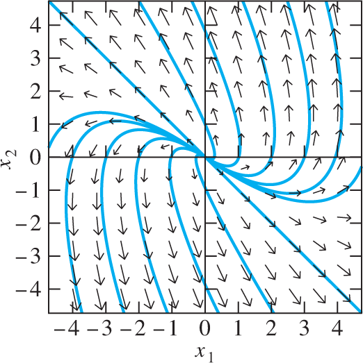
FIGURE 7.6.1.

Direction field and solution curves for the linear system $x_{1}^{′} = x_{1} - 3 x_{2}, x_{2}^{′} = 3 x_{1} + 7 x_{2}$ of Example 3.

Generalized Eigenvectors

The vector $v_{2}$ in Eq. (16) is an example of a generalized eigenvector. If $λ$ is an eigenvalue of the matrix A, then a rank r generalized eigenvector associated with $λ$ is a vector v such that

${(A - λ I)}^{′} v = 0 but {(A - λ I)}^{r - 1} v \neq 0$ (21)

If $r = 1$ , then (21) simply means that v is an eigenvector associated with $λ$ (recalling the convention that the 0th power of a square matrix is the identity matrix). Thus a rank 1 generalized eigenvector is an ordinary eigenvector. The vector $v_{2}$ in (16) is a rank 2 generalized eigenvector (and not an ordinary eigenvector).

The multiplicity 2 method described earlier boils down to finding a pair ${v_{1}, v_{2}}$ of generalized eigenvectors, one of rank 1 and one of rank 2, such that $(A - λ I) v_{2} = v_{1}$ . Higher multiplicity methods involve longer “chains” of generalized eigenvectors. A length k chain of generalized eigenvectors based on the eigenvector $v_{1}$ is a set ${v_{1}, v_{2}, \dots, v_{k}}$ of k generalized eigenvectors such that

$\begin{array}{rcl} (A - λ I) v_{k} & = & v_{k} - 1, \\ (A - λ I) v_{k} - 1 & = & v_{k} - 2, \\ ⋮ \\ (A - λ I) v_{2} & = & v_{1} \end{array}$ (22)

Because $v_{1}$ is an ordinary eigenvector, $(A - λ I) v_{1} = 0$ . Therefore, it follows from (22) that

${(A - λ I)}^{k} v_{k} = 0.$ (23)

If ${v_{1}, v_{2}, v_{3}}$ is a length 3 chain of generalized eigenvectors associated with the multiple eigenvalue $λ$ of the matrix A, then it is easy to verify that three linearly independent solutions of $x ′ = A x$ are given by

$\begin{aligned} x_{1} (t) & = & v_{1} e^{λ t}, \\ x_{2} (t) & = & (v_{1} t + v_{2}) e^{λ t}, \\ x_{3} (t) & = & (\frac{1}{2} v_{1} t^{2} + v_{2} t + v_{3}) e^{λ t} . \end{aligned}$ (24)

For instance, the equations in (22) give

$\begin{array}{c} A v_{3} = v_{2} + λ v_{3}, & A v_{2} = v_{1} + λ v_{2}, & A v_{3} = λ v_{1}, \end{array}$

$\begin{aligned} A x_{3} & = & [\frac{1}{2} A v_{1} t^{2} + A v_{2} t + A v_{3}] e^{λ t} \\ = & [\frac{1}{2} λ v_{1} t^{2} + (v_{1} + λ v_{2}) t + (v_{2} + λ v_{3})] e^{λ t} \\ = & (v_{1} t + v_{2}) e^{λ t} + λ (\frac{1}{2} v_{1} t^{2} + v_{2} t + v_{3}) e^{λ t} \\ = & x_{3}^{′} . \end{aligned}$

Therefore, $x_{3} (t)$ in (24) does, indeed, define a solution of $x ′ = A x$ .

Consequently, in order to “handle” a multiplicity 3 eigenvalue $λ$ , it suffices to find a length 3 chain ${v_{1}, v_{2}, v_{3}}$ of generalized eigenvalues associated with $λ$ . Looking at Eq. (23), we see that we need only find a solution $v_{3}$ of

${(A - λ I)}^{3} v_{3} = 0$

such that the vectors

$v_{2} = (A - λ I) v_{3} and v_{1} = (A - λ I) v_{2}$

are both nonzero (although, as we will see, this is not always possible).

Example 4

Find three linearly independent solutions of the system

$x^{′} = [\begin{array}{r} 0 & 1 & 2 \\ - 5 & - 3 & - 7 \\ 1 & 0 & 0 \end{array}] x .$ (25)

Solution

The characteristic equation of the coefficient matrix in Eq. (25) is

$\begin{aligned} | A - λ I | & = & [\begin{array}{c} - λ & 1 & 2 \\ - 5 & - 3 - λ & - 7 \\ 1 & 0 & - λ \end{array}] \\ = & 1 \cdot [- 7 - 2 \cdot (- 3 - λ)] + (- λ) [(- λ) (- 3 - λ) + 5] \\ = & - λ^{3} - 3 λ^{2} - 3 λ - 1 = - {(λ + 1)}^{3} = 0, \end{aligned}$

and thus A has the eigenvalue $λ = - 1$ of multiplicity 3. The eigenvector equation $(A - λ I) v = 0$ for an eigenvector $v = {[\begin{array}{r} a & b & c \end{array}]}^{T}$ is

$(A + I) v = [\begin{array}{r} 1 & 1 & 2 \\ - 5 & - 2 & - 7 \\ 1 & 0 & 1 \end{array}] [\begin{matrix} a \\ b \\ c \end{matrix}] = [\begin{matrix} 0 \\ 0 \\ 0 \end{matrix}] .$

The third row $a + c = 0$ gives $c = - a$ ; then the first row $a + b + 2 c = 0$ gives $b = a$ . Thus, to within a constant multiple, the eigenvalue $λ = - 1$ has only the single associated eigenvector $v = {[\begin{array}{r} a & a & - a \end{array}]}^{T}$ with $a \neq 0$ , and so the defect of $λ = - 1$ is 2.

To apply the method described here for triple eigenvalues, we first calculate

${(A + I)}^{2} = [\begin{array}{r} 1 & 1 & 2 \\ - 5 & - 2 & - 7 \\ 1 & 0 & 1 \end{array}] [\begin{array}{r} 1 & 1 & 2 \\ - 5 & - 2 & - 7 \\ 1 & 0 & 1 \end{array}] = [\begin{array}{r} - 2 & - 1 & - 3 \\ - 2 & - 1 & - 3 \\ 2 & 1 & 3 \end{array}]$

and

${(A + I)}^{3} = [\begin{array}{r} 1 & 1 & 2 \\ - 5 & - 2 & - 7 \\ 1 & 0 & 1 \end{array}] [\begin{array}{r} - 2 & - 1 & - 3 \\ - 2 & - 1 & - 3 \\ 2 & 1 & - 3 \end{array}] = [\begin{array}{r} 0 & 0 & 0 \\ 0 & 0 & 0 \\ 0 & 0 & 0 \end{array}] .$

Thus any nonzero vector $v_{3}$ will be a solution of the equation ${(A + I)}^{3} v_{3} = 0$ . Beginning with $v_{3} = {[\begin{array}{r} 1 & 0 & 0 \end{array}]}^{T},$ for instance, we calculate

$\begin{aligned} v_{2} & = & (A + I) v_{3} = [\begin{array}{r} 1 & 1 & 2 \\ - 5 & - 2 & - 7 \\ 1 & 0 & 1 \end{array}] [\begin{array}{r} 1 \\ 0 \\ 0 \end{array}] = [\begin{array}{r} 1 \\ - 5 \\ 1 \end{array}], \\ v_{1} & = & (A + I) v_{2} = [\begin{array}{r} 1 & 1 & 2 \\ - 5 & - 2 & - 7 \\ 1 & 0 & 1 \end{array}] [\begin{array}{r} 1 \\ - 5 \\ 1 \end{array}] = [\begin{array}{r} - 2 \\ - 2 \\ - 2 \end{array}] . \end{aligned}$

Note that $v_{1}$ is the previously found eigenvector v with $a = - 2$ ; this agreement serves as a check of the accuracy of our matrix computations.

Thus we have found a length 3 chain ${v_{1}, v_{2}, v_{3}}$ of generalized eigenvectors associated with the triple eigenvalue $λ = - 1$ . Substitution in (24) now yields the linearly independent solutions

$\begin{aligned} x_{1} (t) & = & v_{1} e^{- t} = [\begin{array}{r} - 2 \\ - 2 \\ 2 \end{array}] e^{- t}, \\ x_{2} (t) & = & (v_{1} t + v_{2}) e^{- t} = [\begin{array}{r} - 2 t + 1 \\ - 2 t - 5 \\ 2 t + 1 \end{array}] e^{- t}, \\ x_{3} (t) & = & (\frac{1}{2} v_{1} t^{2} + v_{2} t + v_{3}) e^{- t} = [\begin{array}{c} - t^{2} + t + 1 \\ - t^{2} - 5 t \\ t^{2} + t \end{array}] e^{- t} \end{aligned}$

of the system $x ′ = A x$ .

The General Case

A fundamental theorem of linear algebra states that every $n \times n$ matrix A has n linearly independent generalized eigenvectors. These n generalized eigenvectors may be arranged in chains, with the sum of the lengths of the chains associated with a given eigenvalue $λ$ equal to the multiplicity of $λ$ . But the structure of these chains depends on the defect of $λ$ , and can be quite complicated. For instance, a multiplicity 4 eigenvalue can correspond to

Four length 1 chains (defect 0);
Two length 1 chains and a length 2 chain (defect 1);
Two length 2 chains (defect 2);
A length 1 chain and a length 3 chain (defect 2); or
A length 4 chain (defect 3).

Note that, in each of these cases, the length of the longest chain is at most $d + 1$ , where d is the defect of the eigenvalue. Consequently, once we have found all the ordinary eigenvectors associated with a multiple eigenvalue $λ$ , and therefore know the defect d of $λ$ , we can begin with the equation

${(A - λ I)}^{d + 1} u = 0$ (26)

to start building the chains of generalized eigenvectors associated with $λ$ .

Each length k chain ${v_{1}, v_{2}, \dots, v_{k}}$ of generalized eigenvectors (with $v_{1}$ an ordinary eigenvector associated with $λ$ ) determines a set of k independent solutions of $x ′ = A x$ corresponding to the eigenvalue $λ$ :

$\begin{array}{rcl} x_{1} (t) & = & v_{1} e^{λ t}, \\ x_{2} (t) & = & (v_{1} t + v_{2}) e^{λ t}, \\ x_{3} (t) & = & (\frac{1}{2} v_{1} t + v_{2} t + v_{3}) e^{λ t}, \\ ⋮ \\ x_{k} (t) & = & (\frac{v_{1} t^{k - 1}}{(k - 1)!} + \dots + \frac{v_{k - 2} t^{2}}{2!} + v_{k - 1} t + v_{k}) e^{λ t} . \end{array}$ (27)

Note that (27) reduces to Eqs. (18) through (19) and (24) in the cases $k = 2$ and $k = 3$ , respectively.

To ensure that we obtain n generalized eigenvectors of the $n \times n$ matrix A that are actually linearly independent, and therefore produce a complete set of n linearly independent solutions of $x ′ = A x$ when we amalgamate all the “chains of solutions” corresponding to different chains of generalized eigenvectors, we may rely on the following two facts:

Any chain of generalized eigenvectors constitutes a linearly independent set of vectors.
If two chains of generalized eigenvectors are based on linearly independent eigenvectors, then the union of these two chains is a linearly independent set of vectors (whether the two base eigenvectors are associated with different eigenvalues or with the same eigenvalue).

Example 5

Suppose that the $6 \times 6$ matrix A has two multiplicity 3 eigenvalues $λ_{1} = - 2$ and $λ_{2} = 3$ with defects 1 and 2, respectively. Then $λ_{1}$ must have an associated eigenvector $u_{1}$ and a length 2 chain ${v_{1}, v_{2}}$ of generalized eigenvectors (with the eigenvectors $u_{1}$ and $v_{1}$ being linearly independent), whereas $λ_{2}$ must have a length 3 chain ${w_{1}, w_{2}, w_{3}}$ of generalized eigenvectors based on its single eigenvector $w_{1}$ . The six generalized eigenvectors $u_{1}, v_{1}, v_{2}, w_{1}, w_{2}$ , and $w_{3}$ are then linearly independent and yield the following six independent solutions of $x ′ = A x$ :

$\begin{aligned} x_{1} (t) & = & u_{1} e^{- 2 t}, \\ x_{2} (t) & = & v_{1} e^{- 2 t}, \\ x_{3} (t) & = & (v_{1} t + v_{2}) e^{- 2 t}, \\ x_{4} (t) & = & w_{1} e^{3 t}, \\ x_{5} (t) & = & (w_{1} t + w_{2}) e^{3 t}, \\ x_{6} (t) & = & (\frac{1}{2} w_{1} t^{2} + w_{2} t + w_{3}) e^{3 t} . \end{aligned}$

As Example 5 illustrates, the computation of independent solutions corresponding to different eigenvalues and chains of generalized eigenvalues is a routine matter. The determination of the chain structure associated with a given multiple eigenvalue can be more interesting (as in Example 6).

An Application

Figure 7.6.2 shows two railway cars that are connected with a spring (permanently attached to both cars) and with a damper that exerts opposite forces on the two cars, of magnitude $c (x_{1}^{′} - x_{2}^{′})$ proportional to their relative velocity. The two cars are also subject to frictional resistance forces $c_{1} x_{1}^{′}$ and $c_{2} x_{2}^{′}$ proportional to their respective velocities. An application of Newton’s law $m a = F$ (as in Example 1 of Section 7.1) yields the equations of motion

$\begin{aligned} m_{1} x_{1}^{″} & = & k (x_{2} - x_{1}) - c_{1} x_{1}^{′} - c (x_{1}^{′} - x_{2}^{′}), \\ m_{2} x_{2}^{″} & = & k (x_{1} - x_{2}) - c_{2} x_{2}^{′} - c (x_{2}^{′} - x_{1}^{′}) . \end{aligned}$ (28)

FIGURE 7.6.2.

The railway cars of Example 6.

In terms of the position vector $x (t) = {[\begin{array}{r} x_{1} (t) & x_{2} (t) \end{array}]}^{T},$ these equations can be written in the matrix form

$M x^{″} = K x + R x^{′} .$ (29)

where M and K are mass and stiffness matrices (as in Eqs. (2) and (3) of Section 7.4), and

$R = [\begin{array}{c} - (c + c_{1}) & c \\ c & - (c + c_{2}) \end{array}]$

is the resistance matrix. Unfortunately, because of the presence of the term involving $x ′$ , the methods of Section 7.4 cannot be used.

Instead, we write (28) as a first-order system in the four unknown functions $x_{1} (t), x_{2} (t), x_{3} (t) = x_{1}^{′} (t)$ , and $x_{4} (t) = x_{2}^{′} (t)$ . If $m_{1} = m_{2} = 1$ we get

$x^{′} = A x,$ (30)

where now $x = {[\begin{array}{r} x_{1} & x_{2} & x_{3} & x_{4} \end{array}]}^{T}$ and

$A = [\begin{array}{rrcc} 0 & 0 & 1 & 0 \\ 0 & 0 & 0 & 1 \\ - k & k & - (c + c_{1}) & c \\ k & - k & c & - (c + c_{2}) \end{array}] .$ (31)

Example 6

Two railway cars With $m_{1} = m_{2} = c = 1$ and $k = c_{1} = c_{2} = 2$ , the system in Eq. (30) is

$x^{′} = [\begin{array}{r} 0 & 0 & 1 & 0 \\ 0 & 0 & 0 & 1 \\ - 2 & 2 & - 3 & 1 \\ 2 & - 2 & 1 & - 3 \end{array}] x .$ (32)

It is not too tedious to calculate manually—although a computer algebra system such as Maple, Mathematica, or Matlab is useful here—the characteristic equation

$λ^{4} + 6 λ^{3} + 12 λ^{2} + 8 λ = λ {(λ + 2)}^{2} = 0$

of the coefficient matrix A in Eq. (32). Thus A has the distinct eigenvalue $λ_{0} = 0$ and the triple eigenvalue $λ_{1} = - 2$ .

Case 1: $λ_{0} = 0 .$ The eigenvalue equation $(A - λ I) v = 0$ for the eigenvector $v = {[\begin{array}{c} a & b & c & d \end{array}]}^{T}$ is

$A v = [\begin{array}{r} 0 & 0 & 1 & 0 \\ 0 & 0 & 0 & 1 \\ - 2 & 2 & - 3 & 1 \\ 2 & - 2 & 1 & - 3 \end{array}] [\begin{array}{r} a \\ b \\ c \\ d \end{array}] = [\begin{array}{r} 0 \\ 0 \\ 0 \\ 0 \end{array}] .$

The first two rows give $c = d = 0;$ then the last two rows yield $a = b .$ Thus

$v_{0} = {[\begin{array}{r} 1 & 1 & 0 & 0 \end{array}]}^{T}$

is an eigenvector associated with $λ_{0} = 0$ .

Case 2: $λ_{1} = - 2$ The eigenvalue equation $(A - λ I) v = 0$ is

$(A + 2 I) v = [\begin{array}{r} 2 & 0 & 1 & 0 \\ 0 & 2 & 0 & 1 \\ - 2 & 2 & - 1 & 1 \\ 2 & - 2 & 1 & - 1 \end{array}] [\begin{array}{r} a \\ b \\ c \\ d \end{array}] = [\begin{array}{r} 0 \\ 0 \\ 0 \\ 0 \end{array}] .$

The third and fourth scalar equations here are the differences of the first and second equations, and therefore are redundant. Hence v is determined by the first two equations,

$2 a + c = 0 and 2 b + d = 0.$

We can choose a and b independently, then solve for c and d. Thereby we obtain two eigenvectors associated with the triple eigenvalue $λ_{1} = - 2$ . The choice $a = 1, b = 0$ yields $c = - 2, d = 0$ and thereby the eigenvector

$u_{1} = {[\begin{array}{r} 1 & 0 & - 2 & 0 \end{array}]}^{T} .$

The choice $a = 0, b = 1$ yields $c = 0, d = - 2$ and thereby the eigenvector

$u_{2} = {[\begin{array}{r} 1 & 0 & 0 & - 2 \end{array}]}^{T} .$

Because $λ_{1} = - 2$ has defect 1, we need a generalized eigenvector of rank 2, and hence a nonzero solution $v_{2}$ of the equation

${(A + 2 I)}^{2} v_{2} = [\begin{array}{r} 2 & 2 & 1 & 1 \\ 2 & 2 & 1 & 1 \\ 0 & 0 & 0 & 0 \\ 0 & 0 & 0 & 0 \end{array}] v_{2} = 0.$

Obviously,

$v_{2} = {[\begin{array}{r} 0 & 0 & 1 & - 1 \end{array}]}^{T}$

is such a vector, and we find that

$(A + 2 I) v_{2} = [\begin{array}{r} 2 & 0 & 1 & 0 \\ 0 & 2 & 0 & 1 \\ - 2 & 2 & - 1 & 1 \\ 2 & - 2 & 1 & - 1 \end{array}] [\begin{array}{r} 0 \\ 0 \\ 1 \\ - 1 \end{array}] = [\begin{array}{r} 1 \\ - 1 \\ - 2 \\ 2 \end{array}] = v_{1}$

is nonzero, and therefore is an eigenvector associated with $λ_{1} = - 2$ . Then ${v_{1}, v_{2}}$ is the length 2 chain we need.

The eigenvector $v_{1}$ just found is neither of the two eigenvectors $u_{1}$ and $u_{2}$ found previously, but we observe that $v_{1} = u_{1} - u_{2}$ . For a length 1 chain $w_{1}$ to complete the picture, we can choose any linear combination of $u_{1}$ and $u_{2}$ that is independent of $v_{1}$ . For instance, we could choose either $w_{1} = u_{1}$ or $w_{1} = u_{2}$ . However, we will see momentarily that the particular choice

$w_{1} = u_{1} + u_{2} = {[\begin{array}{r} 1 & 1 & - 2 & - 2 \end{array}]}^{T}$

yields a solution of the system that is of physical interest.

Finally, the chains ${v_{0}}, {w_{1}}$ , and ${v_{1}, v_{2}}$ yield the four independent solutions

$\begin{aligned} x_{1} (t) & = & v_{0} e^{0 \cdot t} = {[\begin{array}{r} 1 & 1 & 0 & 0 \end{array}]}^{T}, \\ x_{2} (t) & = & w_{1} e^{- 2 t} = {[\begin{array}{r} 1 & 1 & - 2 & - 2 \end{array}]}^{T} e^{- 2 t}, \\ x_{3} (t) & = & v_{1} e^{- 2 t} = {[\begin{array}{r} 1 & - 1 & - 2 & 2 \end{array}]}^{T} e^{- 2 t}, \\ x_{4} (t) & = & (v_{1} t + v_{2}) e^{- 2 t} \\ = & {[\begin{array}{r} t & - t & - 2 t + 1 & 2 t - 1 \end{array}]}^{T} e^{- 2 t} \end{aligned}$ (33)

of the system $x ′ = A x$ in (32).

The four scalar components of the general solution

$x (t) = c_{1} x_{1} (t) + c_{2} x_{2} (t) + c_{3} x_{3} (t) + c_{4} x_{4} (t)$

are described by the equations

$\begin{aligned} x_{1} (t) & = & c_{1} + e^{- 2 t} (c_{2} + c_{3} + c_{4} t), \\ x_{2} (t) & = & c_{1} + e^{- 2 t} (c_{2} - c_{3} - c_{4} t), \\ x_{2} (t) & = & e^{- 2 t} (- 2 c_{2} - 2 c_{3} + c_{4} - 2 c_{4} t), \\ x_{2} (t) & = & e^{- 2 t} (- 2 c_{2} + 2 c_{3} - c_{4} + 2 c_{4} t) . \end{aligned}$ (34)

Recall that $x_{1} (t)$ and $x_{2} (t)$ are the position functions of the two masses, whereas $x_{3} (t) = x_{1}^{′} (t)$ and $x_{4} (t) = x_{2}^{′} (t)$ are their respective velocity functions.

For instance, suppose that $x_{1} (0) = x_{2} (0) = 0$ and that $x_{1}^{′} (0) = x_{2}^{′} (0) = v_{0}$ . Then the equations

$\begin{array}{r} x_{1} (0) & = & c_{1} & + & c_{2} & + & c_{3} & = & 0, \\ x_{2} (0) & = & c_{3} & + & c_{2} & - & c_{3} & = & 0, \\ x_{1}^{′} (0) & = & - & 2 c_{2} & - & 2 c_{3} & + & c_{4} & = & v_{0}, \\ x_{2}^{′} (0) & = & - & 2 c_{2} & + & 2 c_{3} & - & c_{4} & = & v_{0} \end{array}$

are readily solved for $c_{1} = \frac{1}{2} v_{0}, c_{2} = - \frac{1}{2} v_{0}$ , and $c_{3} = c_{4} = 0,$ so

$\begin{aligned} x_{1} (t) & = & x_{2} (t) & = & \frac{1}{2} v_{0} (1 - e^{- 2 t}), \\ x_{1}^{′} (t) & = & x_{2}^{′} (t) & = & v_{0} e^{- 2 t} . \end{aligned}$

In this case the two railway cars continue in the same direction with equal but exponentially damped velocities, approaching the displacements $x_{1} = x_{2} = \frac{1}{2} v_{0}$ as $t \to + \infty$ .

It is of interest to interpret physically the individual generalized eigenvector solutions given in (33). The degenerate ( $λ_{0} = 0$ ) solution

$x_{1} (t) = {[\begin{array}{r} 1 & 1 & 0 & 0 \end{array}]}^{T}$

describes the two masses at rest with position functions $x_{1} (t) \equiv 1$ and $x_{2} (t) \equiv 1$ . The solution

$x_{2} (t) = {[\begin{array}{r} 1 & 1 & - 2 & - 2 \end{array}]}^{T} e^{- 2 t}$

corresponding to the carefully chosen eigenvector $w_{1}$ describes damped motions $x_{1} (t) = e^{- 2 t}$ and $x_{2} (t) = e^{- 2 t}$ of the two masses, with equal velocities in the same direction. Finally, the solutions $x_{3} (t)$ and $x_{4} (t)$ resulting from the length 2 chain ${v_{1}, v_{2}}$ both describe damped motion with the two masses moving in opposite directions.

The methods of this section apply to complex multiple eigenvalues just as to real multiple eigenvalues (although the necessary computations tend to be somewhat lengthy). Given a complex conjugate pair $α \pm β i$ of eigenvalues of multiplicity k, we work with one of them (say, $α - β i$ ) as if it were real to find k independent complex-valued solutions. The real and imaginary parts of these complex-valued solutions then provide 2k real-valued solutions associated with the two eigenvalues $λ = α - β i$ and $\overset{̲}{λ} = α + β i$ each of multiplicity k. See Problems 33 and 34.

The Jordan Normal Form

In Section 6.2 we saw that if the $n \times n$ matrix A has a complete set $v_{1}, v_{2}, \dots, v_{n}$ of n linearly independent eigenvectors, then it is similar to a diagonal matrix. In particular,

$P^{- 1} A P = D,$ (35)

where $P = [\begin{array}{r} v_{1} & v_{2} & \dots & v_{n} \end{array}]$ and the diagonal elements of the diagonal matrix D are the corresponding eigenvalues $λ_{1}, λ_{2}, \dots, λ_{n}$ (not necessarily distinct). This result is a special case of the following general theorem, a proof of which can be found in Appendix B of Gilbert Strang, Linear Algebra and Its Applications (4th edition, Brooks Cole, 2006).

If the Jordan block $J_{i}$ in (37) is of size $k \times k$ , then it corresponds to a length k chain of generalized eigenvectors based on the (ordinary) eigenvector $v_{i}$ . If all these generalized eigenvectors are arranged as column vectors in proper order corresponding to the appearance of the Jordan blocks in (36), the result is a nonsingular $n \times n$ matrix Q such that

$Q^{- 1} A Q = J .$ (38)

The block-diagonal matrix J such that $A = Q J Q^{- 1}$ is called the Jordan normal form of the matrix A and is unique [except for the order of appearance of the Jordan blocks in (36)].

Example 7

In Example 3 we saw that the matrix

$A = [\begin{array}{r} 1 & - 3 \\ 3 & 7 \end{array}]$

has the single eigenvalue $λ = 4$ and the associated length 2 chain of generalized eigenvectors ${v_{1}, v_{2}}$ , where $v_{1} = {[\begin{array}{r} - 3 & 3 \end{array}]}^{T}$ and $v_{2} = {[\begin{array}{r} 1 & 0 \end{array}]}^{T},$ based on the eigenvector $v_{1} = A v_{2}$ . If we define

$Q = [\begin{array}{r} v_{1} & v_{2} \end{array}] = [\begin{array}{r} - 3 & 1 \\ 3 & 0 \end{array}],$

then we find that the Jordan normal form of A is

$J = Q^{- 1} A Q = [\begin{array}{r} 4 & 1 \\ 0 & 4 \end{array}] .$

Here $J = J_{1}$ is a single $2 \times 2$ Jordan block corresponding to the single eigenvalue $λ = 4$ of A.

Example 8

In Example 6 we saw that the matrix

$A = [\begin{array}{r} 0 & 0 & 1 & 0 \\ 0 & 0 & 0 & 1 \\ - 2 & 2 & - 3 & 1 \\ 2 & - 2 & 1 & - 3 \end{array}]$

has the distinct eigenvalue $λ_{1} = 0$ corresponding to the eigenvector

$v_{1} = {[\begin{array}{c} 1 & 1 & 0 & 0 \end{array}]}^{T}$

and the triple eigenvalue $λ_{2} = - 2$ corresponding both to the eigenvector $v_{2} = {[\begin{array}{c} 1 & 0 & - 2 & 0 \end{array}]}^{T}$ and to the length 2 chain of generalized eigenvectors ${v_{3}, v_{4}}$ with $v_{3} = {[\begin{array}{c} 1 & - 1 & - 2 & 2 \end{array}]}^{T}$ and $v_{4} = {[\begin{array}{c} 0 & 0 & 1 & - 1 \end{array}]}^{T},$ such that $v_{3} = (A + 2 I) v_{4}$ . If we define

$Q = [\begin{array}{c} v_{1} & v_{2} & v_{3} & v_{4} \end{array}] = [\begin{array}{r} 1 & 1 & 1 & 0 \\ 1 & 0 & - 1 & 0 \\ 0 & - 2 & - 2 & 1 \\ 0 & 0 & 2 & - 1 \end{array}],$

then (using a computer algebra system to ease the labor of calculation) we find that the Jordan normal form of A is

$J = Q^{- 1} A Q = [\begin{array}{r} 0 & 0 & 0 & 0 \\ 0 & - 2 & 0 & 0 \\ 0 & 0 & - 2 & 1 \\ 0 & 0 & 0 & - 2 \end{array}] .$

Here we see the $1 \times 1$ Jordan block $J_{1} = [\begin{array}{r} 0 \end{array}]$ corresponding to the eigenvalue $λ_{1} = 0$ of A, as well as the two Jordan blocks $J_{2} = [\begin{array}{r} - 2 \end{array}]$ and $J_{3} = [\begin{array}{r} - 2 & 1 \\ 0 & - 2 \end{array}]$ corresponding to the two linearly independent eigenvectors $v_{2}$ and $v_{3}$ associated with the eigenvalue $λ_{2} = - 2$ .

The General Cayley-Hamilton Theorem

In Section 6.3, we showed that every diagonalizable matrix A satisfies its characteristic equation $p (λ) = | A - λ I | = 0$ , that is, $p (A) = 0$ . We can now use the Jordan normal form to show that this is true whether or not A is diagonalizable.

If $J = Q^{- 1} A Q$ is the Jordan normal form of the matrix A, then $p (A) = Q p (J) Q^{- 1}$ , just as in the conclusion to the proof of Theorem 1 in Section 6.3. It therefore suffices to show that $p (J) = 0$ . If the Jordan blocks $J_{1}, J_{2}, \dots, J_{s}$ in (36) have sizes $k_{1}, k_{2}, \dots, k_{s}$ —that is, $J_{i}$ is a $k_{i} \times k_{i}$ matrix—and corresponding eigenvalues $λ_{1}, λ_{2}, \dots, λ_{s}$ (respectively), then

$p (λ) = {(λ_{1} - λ)}^{k_{1}} {(λ_{2} - λ)}^{k_{2}} \dots {(λ_{s} - λ)}^{k_{s}},$

and so

$p (J) = {(λ_{1} I - J)}^{k_{1}} {(λ_{2} I - J)}^{k_{2}} \dots {(λ_{s} I - J)}^{k_{s}} .$ (39)

Now p(J) has the same block-diagonal structure as J itself, and we see from (39) that the ith block of p(J) involves the factor

${(λ_{i} I - J_{i})}^{k_{i}} = {[\begin{array}{c} 0 & - 1 & 0 & \dots & 0 \\ 0 & 0 & - 1 & \dots & 0 \\ ⋮ & ⋮ & ⋱ & ⋱ & ⋮ \\ 0 & 0 & \dots & 0 & - 1 \\ 0 & 0 & 0 & \dots & 0 \end{array}]}^{k_{i}},$

where the $k_{i} \times k_{i}$ matrix $λ_{i} I - J_{i}$ has all elements zero except on its first superdiagonal. It is easily seen that ${(λ_{i} I - J_{i})}^{2}$ then has nonzero elements only on its second superdiagonal; ${(λ_{i} I - J_{i})}^{3}$ has nonzero elements only on its third superdiagonal; and so on, in turn, until we see that ${(λ_{i} I - J_{i})}^{k_{i}} = 0$ . Hence it follows from (39) that the ith block of p(J) is the $k_{i} \times k_{i}$ zero matrix. This being true for each $i = 1, 2, \dots, s$ , we conclude that $p (J) = 0$ , as desired. This completes the proof of the general case of the Cayley-Hamilton theorem.

7.6 Problems

Find general solutions of the systems in Problems 1 through 22. In Problems 1 through 6, use a computer system or graphing calculator to construct a direction field and typical solution curves for the given system.

$x^{′} = [\begin{array}{r} - 2 & 1 \\ - 1 & - 4 \end{array}] x$
$x^{′} = [\begin{array}{r} 3 & - 1 \\ 1 & 1 \end{array}] x$
$x^{′} = [\begin{array}{r} 1 & - 2 \\ 2 & 5 \end{array}] x$
$x^{′} = [\begin{array}{r} 3 & - 1 \\ 1 & 5 \end{array}] x$
$x^{′} = [\begin{array}{r} 7 & 1 \\ - 4 & 3 \end{array}] x$
$x^{′} = [\begin{array}{r} 1 & - 4 \\ 4 & 9 \end{array}] x$
$x^{′} = [\begin{array}{r} 2 & 0 & 0 \\ - 7 & 9 & 7 \\ 0 & 0 & 2 \end{array}] x$
$x^{′} = [\begin{array}{r} 25 & 12 & 0 \\ - 18 & - 5 & 0 \\ 6 & 6 & 13 \end{array}] x$
$x^{′} = [\begin{array}{r} - 19 & 12 & 84 \\ 0 & 5 & 0 \\ - 8 & 4 & 33 \end{array}] x$
$x^{′} = [\begin{array}{r} - 13 & 40 & - 48 \\ - 8 & 23 & - 24 \\ 0 & 0 & 3 \end{array}] x$
$x^{′} = [\begin{array}{r} - 3 & 0 & - 4 \\ - 1 & - 1 & - 1 \\ 1 & 0 & 1 \end{array}] x$
$x^{′} = [\begin{array}{r} - 1 & 0 & 1 \\ 0 & - 1 & 1 \\ 1 & - 1 & - 1 \end{array}] x$
$x^{′} = [\begin{array}{r} - 1 & 0 & 1 \\ 0 & 1 & - 4 \\ 0 & 1 & - 3 \end{array}] x$
$x^{′} = [\begin{array}{r} 0 & 0 & 1 \\ - 5 & - 1 & - 5 \\ 4 & 1 & - 2 \end{array}] x$
$x^{′} = [\begin{array}{r} - 2 & - 9 & 0 \\ 1 & 4 & 0 \\ 1 & 3 & 1 \end{array}] x$
$x^{′} = [\begin{array}{r} 1 & 0 & 0 \\ - 2 & - 2 & - 3 \\ 2 & 3 & 4 \end{array}] x$
$x^{′} = [\begin{array}{r} 1 & 0 & 0 \\ 18 & 7 & 4 \\ - 27 & - 9 & - 5 \end{array}] x$
$x^{′} = [\begin{array}{r} 1 & 0 & 0 \\ 1 & 3 & 1 \\ - 2 & - 4 & - 1 \end{array}] x$
$x^{′} = [\begin{array}{r} 1 & - 4 & 0 & - 2 \\ 0 & 1 & 0 & 0 \\ 6 & - 12 & - 1 & - 6 \\ 0 & - 4 & 0 & - 1 \end{array}] x$
$x^{′} = [\begin{array}{r} 2 & 1 & 0 & 1 \\ 0 & 2 & 1 & 0 \\ 0 & 0 & 2 & 1 \\ 0 & 0 & 0 & 2 \end{array}] x$
$x^{′} = [\begin{array}{r} - 1 & - 4 & 0 & 0 \\ 1 & 3 & 0 & 0 \\ 1 & 2 & 1 & 0 \\ 0 & 1 & 0 & 1 \end{array}] x$
$x ′ = [\begin{array}{r} 1 & 3 & 7 & 0 \\ 0 & - 1 & - 4 & 0 \\ 0 & 1 & 3 & 0 \\ 0 & - 6 & - 14 & 1 \end{array}] x$

In Problems 23 through 32 the eigenvalues of the coefficient matrix A are given. Find a general solution of the indicated system $x ′ = A x$ . Especially in Problems 29 through 32, use of a computer algebra system (as in the application material for this section) may be useful.

$x^{′} = [\begin{array}{r} 39 & 8 & - 16 \\ - 36 & - 5 & 16 \\ 72 & 16 & - 29 \end{array}] x; λ = - 1, 3, 3,$
$x^{′} = [\begin{array}{r} 28 & 50 & 100 \\ 15 & 33 & 60 \\ - 15 & - 30 & - 57 \end{array}] x; λ = - 2, 3, 3$
$x^{′} = [\begin{array}{r} - 2 & 17 & 4 \\ - 1 & 6 & 1 \\ 0 & 1 & 2 \end{array}] x; λ = 2, 2, 2$
$x^{′} = [\begin{array}{r} 5 & - 1 & 1 \\ 1 & 3 & 0 \\ - 3 & 2 & 1 \end{array}] x; λ = 3, 3, 3$
$x^{′} = [\begin{array}{r} - 3 & 5 & - 5 \\ 3 & - 1 & 3 \\ 8 & - 8 & 10 \end{array}] x; λ = 2, 2, 2$
$x^{′} = [\begin{array}{r} - 15 & - 7 & 4 \\ 34 & 16 & - 11 \\ 17 & 7 & 5 \end{array}] x; λ = 2, 2, 2$
$x^{′} = [\begin{array}{r} - 1 & 1 & 1 & - 2 \\ 7 & - 4 & - 6 & 11 \\ 5 & - 1 & 1 & 3 \\ 6 & - 2 & - 2 & 6 \end{array}] x; λ = - 1, - 1, 2, 2$
$x^{′} = [\begin{array}{r} 2 & 1 & - 2 & 1 \\ 0 & 3 & - 5 & 3 \\ 0 & - 13 & 22 & - 12 \\ 0 & - 27 & 45 & - 25 \end{array}] x; λ = - 1, - 1, 2, 2$
$x^{′} = [\begin{array}{r} 35 & - 12 & - 4 & 30 \\ 22 & - 8 & 3 & 19 \\ - 10 & 3 & 0 & - 9 \\ - 27 & 9 & - 3 & - 23 \end{array}] x; λ = 1, 1, 1, 1$
$x^{′} = [\begin{array}{r} 11 & - 1 & 26 & 6 & - 3 \\ 0 & 3 & 0 & 0 & 0 \\ - 9 & 3 & - 24 & - 6 & 3 \\ 3 & 0 & 9 & 5 & - 1 \\ - 48 & - 3 & - 138 & - 30 & 18 \end{array}] x; λ = 2, 2, 3, 3, 3$
The characteristic equation of the coefficient matrix A of the system

$x^{′} = [\begin{array}{r} 3 & - 4 & 1 & 0 \\ 4 & 3 & 0 & 1 \\ 0 & 0 & 3 & - 4 \\ 0 & 0 & 4 & 3 \end{array}] x$

is

$ϕ (λ) = {(λ^{2} - 6 λ + 25)}^{2} = 0.$

Therefore, A has the repeated complex conjugate pair $3 \pm 4 i$ of eigenvalues. First show that the complex vectors

$v_{1} = {[\begin{array}{r} 1 & i & 0 & 0 \end{array}]}^{T} and v_{2} = {[\begin{array}{r} 0 & 0 & 1 & i \end{array}]}^{T}$

form a length 2 chain ${v_{1}, v_{2}}$ associated with the eigenvalue $λ = 3 - 4 i$ . Then calculate the real and imaginary parts of the complex-valued solutions

$v_{1} e^{λ t} and (v_{1} t + v_{2}) e^{λ t}$

to find four independent real-valued solutions of $x ′ = A x$ .
The characteristic equation of the coefficient matrix A of the system

$x^{′} = [\begin{array}{r} 2 & 0 & - 8 & - 3 \\ - 18 & - 1 & 0 & 0 \\ - 9 & - 3 & - 25 & - 9 \\ 33 & 10 & 90 & 32 \end{array}] x$

is

$ϕ (λ) = {(λ^{2} - 4 λ + 13)}^{2} = 0.$

Therefore, A has the repeated complex conjugate pair $2 \pm 3 i$ of eigenvalues. First show that the complex vectors

$\begin{aligned} v_{1} & = & {[\begin{array}{r} - i & 3 + 3 i & 0 & - 1 \end{array}]}^{T}, \\ v_{2} & = & {[\begin{array}{r} 3 & - 10 + 9 i & - i & 0 \end{array}]}^{T} \end{aligned}$

form a length 2 chain ${v_{1}, v_{2}}$ associated with the eigenvalue $λ = 2 + 3 i$ . Then calculate (as in Problem 33) four independent real-valued solutions of $x ′ = A x$ .
Railway cars Find the position functions $x_{1} (t)$ and $x_{2} (t)$ of the railway cars of Fig. 7.5.2 if the physical parameters are given by

$m_{1} = m_{2} = c_{1} = c_{2} = c = k = 1$

and the initial conditions are

$x_{1} (0) = x_{2} (0) = 0, x_{1}^{′} (0) = x_{2}^{′} (0) = v_{0}$

How far do the cars travel before stopping?
Railway cars Repeat Problem 35 under the assumption that car 1 is shielded from air resistance by car 2, so now $c_{1} = 0$ . Show that, before stopping, the cars travel twice as far as those of Problem 35.

37–46. Use the method of Examples 7 and 8 to find the Jordan normal form J of each coefficient matrix A given in Problems 23 through 32 (respectively).

7.6 Application Defective Eigenvalues and Generalized Eigenvectors

A typical computer algebra system can calculate both the eigenvalues of a given matrix A and the linearly independent (ordinary) eigenvectors associated with each eigenvalue. For instance, consider the $4 \times 4$ matrix

$A = [\begin{array}{r} 35 & - 12 & 4 & 30 \\ 22 & - 8 & 3 & 19 \\ - 10 & 3 & 0 & - 9 \\ - 27 & 9 & - 3 & - 23 \end{array}]$ (1)

of Problem 31 in this section. When the matrix A has been entered, the Maple calculation

with(linalg): eigenvectors(A);
[1, 4, {[-1, 0, 1, 1], [0, 1, 3, 0]}]

or the Mathematica calculation

Eigensystem[A]
{{1,1,1,1},
{{-3,-1,0,3}, {0,1,3,0}, {0,0,0,0}, {0,0,0,0}}}

reveals that the matrix A in Eq. (1) has the single eigenvalue $λ = 1$ of multiplicity 4 with only two independent associated eigenvectors $v_{1}$ and $v_{2}$ . The Matlab command

[V, D] = eig(sym(A))

provides the same information. The eigenvalue $λ = 1$ therefore has defect $d = 2$ . If $B = A - (1) I$ , you should find that $B^{2} \neq 0$ but $B^{3} = 0$ . If

$u_{1} = {[1 0 0 0]}^{T}, u_{2} = B u_{1}, u_{3} = B u_{2},$

then ${u_{1}, u_{2}, u_{3}}$ should be a length 3 chain of generalized eigenvectors based on the ordinary eigenvector $u_{3}$ (which should be a linear combination of the original eigenvectors $v_{1}$ and $v_{2}$ ). Use your computer algebra system to carry out this construction, and finally write four linearly independent solutions of the linear system $x ′ = A x$ .

For a more exotic matrix to investigate, consider the Matlab’s gallery(5) example matrix

$A = [\begin{array}{r} - 9 & 11 & - 21 & 63 & - 252 \\ 70 & - 69 & 141 & - 421 & 1684 \\ - 575 & 575 & - 1149 & 3451 & - 13801 \\ 3891 & - 3891 & 7782 & - 23345 & 93365 \\ 1024 & - 1024 & 2048 & - 6144 & 24572 \end{array}] .$ (2)

Use appropriate commands like those illustrated here to show that A has a single eigenvalue $λ = 0$ of multiplicity 5 and defect 4. Noting that $A - (0) I = A$ , you should find that $A^{4} \neq 0$ but that $A^{5} = 0$ . Hence calculate the vectors

$u_{1} = {[1 0 0 0 0]}^{T}, u_{2} = A u_{1}, u_{3} = A u_{2}, u_{4} = A u_{3}, u_{5} = A u_{4} .$

You should find that $u_{5}$ is a nonzero vector such that $A u_{5} = 0$ , and is therefore an (ordinary) eigenvector of A associated with the eigenvalue $λ = 0$ . Thus ${u_{1}, u_{2}, u_{3}, u_{4}, u_{5}}$ is a length 5 chain of generalized eigenvectors of the matrix A in Eq. (2), and you can finally write five linearly independent solutions of the linear system $x ′ = A x$ .

..................Content has been hidden....................

You can't read the all page of ebook, please click here login for view all page.

Table of Contents for 7.6 Multiple Eigenvalue Solutions

Create new playlist

Sign In

Sign Up

Table of Contents for
7.6 Multiple Eigenvalue Solutions