
10.2 Transformation of Initial Value Problems
We now discuss the application of Laplace transforms to solve a linear differential equation with constant coefficients, such as
with given initial conditions x(0)=x0
it involves the transforms of the derivatives x′
The function f is called piecewise smooth on the bounded interval [a, b] if it is piecewise continuous on [a, b] and differentiable except at finitely many points, with f′(t)

FIGURE 10.2.1.
The discontinuities of f′
The main idea of the proof of Theorem 1 is exhibited best by the case in which f′(t)
Because of (3), the integrated term e−stf(t)
Solution of Initial Value Problems
In order to transform Eq. (1), we need the transform of the second derivative as well. If we assume that g(t)=f′(t)
and thus
![]()
A repetition of this calculation gives
After finitely many such steps we obtain the following extension of Theorem 1.
Example 1
Solve the initial value problem
Solution
With the given initial values, Eqs. (4) and (5) yield
and
where (according to our convention about notation) X(s) denotes the Laplace transform of the (unknown) function x(t). Hence the transformed equation is
which we quickly simplify to
Thus
By the method of partial fractions (of integral calculus), there exist constants A and B such that
and multiplication of both sides of this equation by (s−3)(s+2)
If we substitute s=3,
Because L−1{1/(s−a)}=eat,
is the solution of the original initial value problem. Note that we did not first find the general solution of the differential equation. The Laplace transform method directly yields the desired particular solution, automatically taking into account—via Theorem 1 and its corollary—the given initial conditions.
Remark
In Example 1 we found the values of the partial-fraction coefficients A and B by the “trick” of separately substituting the roots s=3
that resulted from clearing fractions. In lieu of any such shortcut, the “sure-fire” method is to collect coefficients of powers of s on the right-hand side,
Then upon equating coefficients of terms of like degree, we get the linear equations
which are readily solved for the same values A=35
Example 2
Forced mass-spring system Solve the initial value problem
Such a problem arises in the motion of a mass-and-spring system with external force, as shown in Fig. 10.2.2.
Solution
Because both initial values are zero, Eq. (5) yields L{x″(t)}=s2X(s).

FIGURE 10.2.2.
A mass–and–spring system satisfying the initial value problem in Example 2. The mass is initially at rest in its equilibrium position.
Therefore,
The method of partial fractions calls for
The sure-fire approach would be to clear fractions by multiplying both sides by the common denominator, and then collect coefficients of powers of s on the right-hand side. Equating coefficients of like powers on the two sides of the resulting equation would then yield four linear equations that we could solve for A, B, C, and D.
However, here we can anticipate that A=C=0,
When we equate coefficients of like powers of s we get the linear equations
which are readily solved for B=35
Because L{sin 2t}=2/(s2+4)
Figure 10.2.3 shows the graph of this period 2π

FIGURE 10.2.3.
The position function x(t) in Example 2.
Examples 1 and 2 illustrate the solution procedure that is outlined in Fig. 10.2.4.

FIGURE 10.2.4.
Using the Laplace transform to solve an initial value problem.
Linear Systems
Laplace transforms are used frequently in engineering problems to solve linear systems in which the coefficients are all constants. When initial conditions are specified, the Laplace transform reduces such a linear system of differential equations to a linear system of algebraic equations in which the unknowns are the transforms of the solution functions. As Example 3 illustrates, the technique for a system is essentially the same as for a single linear differential equation with constant coefficients.
Example 3
Dual mass-spring system Solve the system
subject to the initial conditions
Thus the force f(t)=40 sin 3t
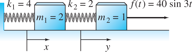
FIGURE 10.2.5.
A mass–and–spring system satisfying the initial value problem in Example 3. Both masses are initially at rest in their equilibrium positions.
Solution
We write X(s)=L{x(t)}
Because L{sin 3t}=3/(s2+9),
Thus the transformed system is
The determinant of this pair of linear equations in X(s) and Y(s) is
and we readily solve—using Cramer’s rule, for instance—the system in (10) for
and
The partial fraction decompositions in Eqs. (11a) and (11b) are readily found using the method of Example 2. For instance, noting that the denominator factors are linear in s2,
and it follows that
Substitution of s2=−1
At any rate, the inverse Laplace transforms of the expressions in Eqs. (11a) and (11b) give the solution
Figure 10.2.6 shows the graphs of these two period 2π

FIGURE 10.2.6.
The position functions x(t) and y(t) in Example 3.
The Transform Perspective
Let us regard the general constant-coefficient second-order equation as the equation of motion
of the familiar mass–spring–dashpot system (Fig. 10.2.7). Then the transformed equation is

FIGURE 10.2.7.
A mass–spring–dashpot system with external force f(t).
Note that Eq. (13) is an algebraic equation—indeed, a linear equation—in the “unknown” X(s). This is the source of the power of the Laplace transform method:
If we solve Eq. (13) for X(s), we get
where
Note that Z(s) depends only on the physical system itself. Thus Eq. (14) presents X(s)=L{x(t)}
of the steady periodic solution and the transient solution, respectively. The only potential difficulty in finding these solutions is in finding the inverse Laplace transform of the right-hand side in Eq. (14). Much of the remainder of this chapter is devoted to finding Laplace transforms and inverse transforms. In particular, we seek those methods that are sufficiently powerful to enable us to solve problems that—unlike those in Examples 1 and 2—cannot be solved readily by the methods of Chapter 5.
Additional Transform Techniques
Example 4
Show that
Solution
If f(t)=teat,
It follows from the linearity of the transform that
Hence
because L{eat}=1/(s−a)
Example 5
Find L{tsin kt}
Solution
Let f(t)=tsin kt.
The derivative involves the new function tcos kt,
But L{f″(t)}=s2L{f(t)}
Finally, we solve this equation for
This procedure is considerably more pleasant than the alternative of evaluating the integral
Examples 4 and 5 exploit the fact that if f(0)=0,
Proof:
Because f is piecewise continuous, the fundamental theorem of calculus implies that
is continuous and that g′(t)=f(t)
so g(t) is of exponential order as t→+∞.
Now g(0)=0,
which completes the proof.
Example 6
Find the inverse Laplace transform of
Solution
In effect, Eq. (18) means that we can delete a factor of s from the denominator, find the inverse transform of the resulting simpler expression, and finally integrate from 0 to t (to “correct” for the missing factor s). Thus
We now repeat the technique to obtain
This technique is often a more convenient way than the method of partial fractions for finding an inverse transform of a fraction of the form P(s)/[snQ(s)]
Proof of Theorem 1:
We conclude this section with the proof of Theorem 1 in the general case in which f′
exists and also need to find its value. With b fixed, let t1,t2,…,tk−1
Now the first summation
in (19) telescopes down to −f(t0)+e−stkf(tk)=−f(0)+e−sbf(b),
But from Eq. (3) we get
if s>c.
Extension of Theorem 1
Now suppose that the function f is only piecewise continuous (instead of continuous), and let t1,t2,t3,…
that may not agree with the actual values f(tn−1)
where
denotes the (finite) jump in f(t) at t=tn.
of L{f′(t)}=sF(s)−f(0)
Example 7
Let f(t)=1+〚t〛

FIGURE 10.2.8.
The graph of the unit staircase function of Example 7.
so the Laplace transform of f(t) is
In the last step we used the formula for the sum of a geometric series,
with x=e−s<1
10.2 Problems
Use Laplace transforms to solve the initial value problems in Problems 1 through 16.
x″+4x=0; x(0)=5, x′(0)=0
x′′+4x=0; x(0)=5, x'(0)=0 x″+9x=0; x(0)=3, x′(0)=4
x′′+9x=0; x(0)=3, x'(0)=4 x″−x′−2x=0; x(0)=0, x′(0)=2
x′′−x'−2x=0; x(0)=0, x'(0)=2 x″+8x′+15x=0; x(0)=2, x′(0)=−3
x′′+8x'+15x=0; x(0)=2, x'(0)=−3 x″+x=sin 2t; x(0)=0=x′(0)
x′′+x=sin 2t; x(0)=0=x'(0) x″+4x=cos t; x(0)=0=x′(0)
x′′+4x=cos t; x(0)=0=x'(0) x″+x=cos 3t; x(0)=1, x′(0)=0
x′′+x=cos 3t; x(0)=1, x'(0)=0 x″+9x=1; x(0)=0=x′(0)
x′′+9x=1; x(0)=0=x'(0) x″+4x′+3x=1; x(0)=0=x′(0)
x′′+4x'+3x=1; x(0)=0=x'(0) x″+3x′+2x=t; x(0)=0, x′(0)=2
x′′+3x'+2x=t; x(0)=0, x'(0)=2 x′=2x+y, y′=6x+3y; x(0)=1, y(0)=−2
x'=2x+y, y'=6x+3y; x(0)=1, y(0)=−2 x′=x+2y, y′=x+e−t; x(0)=y(0)=0
x'=x+2y, y'=x+e−t; x(0)=y(0)=0 x′+2y′+x=0, x′−y′+y=0; x(0)=0, y(0)=1
x'+2y'+x=0, x'−y'+y=0; x(0)=0, y(0)=1 x″+2x+4y=0, y″+x+2y=0; x(0)=y(0)=0, x′(0)=y′(0)=−1
x′′+2x+4y=0, y′′+x+2y=0; x(0)=y(0)=0, x'(0)=y'(0)=−1 x″+x′+y′+2x−y=0, y″+x′+y′+4x−2y=0; x(0)=y(0)=1, x′(0)=y′(0)=0
x′′+x'+y'+2x−y=0, y′′+x'+y'+4x−2y=0; x(0)=y(0)=1, x'(0)=y'(0)=0 x′=x+z, y′=x+y, z′=−2x−z; x(0)=1, y(0)=0; z(0)=0
x'=x+z, y'=x+y, z'=−2x−z; x(0)=1, y(0)=0; z(0)=0
Apply Theorem 2 to find the inverse Laplace transforms of the functions in Problems 17 through 24.
F(s)=1s(s−3)
F(s)=1s(s−3) F(s)=3s(s+5)
F(s)=3s(s+5) F(s)=1s(s2+4)
F(s)=1s(s2+4) F(s)=2s+1s(s2+9)
F(s)=2s+1s(s2+9) F(s)=1s2(s2+1)
F(s)=1s2(s2+1) F(s)=1s(s2−9)
F(s)=1s(s2−9) F(s)=1s2(s2−1)
F(s)=1s2(s2−1) F(s)=1s(s+1)(s+2)
F(s)=1s(s+1)(s+2) Apply Theorem 1 to derive L{sin kt}
L{sin kt} from the formula for L{cos kt}L{cos kt} .Apply Theorem 1 to derive L{coshkt}
L{coshkt} from the formula for L{sinhkt}L{sinhkt} .Apply Theorem 1 to show that
L{tneat}=ns−aL{tn−1eat}.L{tneat}=ns−aL{tn−1eat}. Deduce that L{tneat}=n!/(s−a)n+1
L{tneat}=n!/(s−a)n+1 for n=1, 2, 3,….n=1, 2, 3,….
Apply Theorem 1 as in Example 5 to derive the Laplace transforms in Problems 28 through 30.
L{tcos kt}=s2−k2(s2+k2)2
L{tcos kt}=s2−k2(s2+k2)2 L{tsinhkt}=2ks(s2−k2)2
L{tsinhkt}=2ks(s2−k2)2 L{tcoshkt}=s2+k2(s2−k2)2
L{tcoshkt}=s2+k2(s2−k2)2 Apply the results in Example 5 and Problem 28 to show that
L−1{1(s2+k2)2}=12k3(sinkt−ktcoskt).L−1{1(s2+k2)2}=12k3(sinkt−ktcoskt).
Apply the extension of Theorem 1 in Eq. (22) to derive the Laplace transforms given in Problems 32 through 37.
L{u(t−a)}=s−1e−as
L{u(t−a)}=s−1e−as for a>0a>0 .If f(t)=1
f(t)=1 on the interval [a, b] (where 0<a<b0<a<b ) and f(t)=0f(t)=0 otherwise, thenL{f(t)}=e−as−e−bss.L{f(t)}=e−as−e−bss. If f(t)=(−1)〚t〛
f(t)=(−1)〚t〛 is the square-wave function whose graph is shown in Fig. 10.2.9, thenL{f(t)}=1stanhs2.L{f(t)}=1stanhs2. (Suggestion: Use the geometric series.)

FIGURE 10.2.9.
The graph of the square-wave function of Problem 34.
If f(t) is the unit on—off function whose graph is shown in Fig. 10.2.10, then
L{f(t)}=1s(1+e−s).L{f(t)}=1s(1+e−s). 
FIGURE 10.2.10.
The graph of the on–off function of Problem 35.
If g(t) is the triangular wave function whose graph is shown in Fig. 10.2.11, then
L{g(t)}=1s2tanhs2.L{g(t)}=1s2tanhs2. 
FIGURE 10.2.11.
The graph of the triangular wave function of Problem 36.
If f(t) is the sawtooth function whose graph is shown in Fig. 10.2.12, then
L{f(t)}=1s2−e−ss(1−e−s).L{f(t)}=1s2−e−ss(1−e−s). (Suggestion: Note that f′(t)≡1
f'(t)≡1 where it is defined.)
FIGURE 10.2.12.
The graph of the sawtooth function of Problem 37.
10.2 Application Transforms of Initial Value Problems
The typical computer algebra system knows Theorem 1 and its corollary, hence can transform not only functions (as in the Section 10.1 application), but also entire initial value problems. We illustrate the technique here with Mathematica and in the Section 10.3 application with Maple. Consider the initial value problem
of Example 2. First we define the differential equation with its initial conditions, then load the Laplace transform package.
de = x″ [t] + 4* x[t] == Sin[3* t]
inits = {x[0] −>−> 0,x −>−> 0}The Laplace transform of the differential equation is given by
DE = LaplaceTransform[ de, t, s ]The result of this command—which we do not show explicitly here—is a linear (algebraic) equation in the as yet unknown LaplaceTransform[x[t],t,s]. We proceed to solve for this transform X(s) of the unknown function x(t) and substitute the initial conditions.
X = Solve[DE, LaplaceTransform[x[t],t,s]]
X = X // Last // Last // Last
X = X /. initsFinally we need only compute an inverse transform to find x(t).
x = InverseLaplaceTransform[X,s,t]x /. {Cos[t] Sin[t] −>−> 1/2 Sin[2t]}// ExpandOf course we could probably get this result immediately with DSolve, but the intermediate output generated by the steps shown here can be quite instructive. You can try it for yourself with the initial value problems in Problems 1 through 16.