
7 Linear Systems of Differential Equations
7.1 First-Order Systems and Applications
In Chapters 1 and 5 we discussed methods for solving an ordinary differential equation that involves only one dependent variable. Many applications, however, require the use of two or more dependent variables, each a function of a single independent variable (typically time). Such a problem leads naturally to a system of simultaneous ordinary differential equations. We will usually denote the independent variable by t and the dependent variables (the unknown functions of t) by or by x, y, z, Primes will indicate derivatives with respect to t.
We will restrict our attention to systems in which the number of equations is the same as the number of dependent variables (unknown functions). For instance, a system of two first-order equations in the dependent variables x and y has the general form
where the functions f and g are given. A solution of this system is a pair x(t), y(t) of functions of t that satisfy both equations identically over some interval of values of t.
For an example of a second-order system, consider a particle of mass m that moves in space under the influence of a force field F that depends on time t, the position (x(t), y(t), z(t)) of the particle, and its velocity Writing Newton’s law componentwise, we get the system
of three second-order equations with independent variable t and dependent variables x, y, z; the three right-hand side functions are the components of the vector-valued function F.
Initial Applications
Examples 1 and 2 further illustrate how systems of differential equations arise naturally in scientific problems.
Example 1
Dual mass-spring system Consider the system of two masses and two springs shown in Fig. 7.1.1, with a given external force f(t) acting on the right-hand mass We denote by x(t) the displacement (to the right) of the mass from its static equilibrium position [when the system is motionless and in equilibrium and ] and by y(t) the displacement of the mass from its static position. Thus the two springs are neither stretched nor compressed when x and y are zero.

FIGURE 7.1.1.
The mass-and-spring system of Example 1.
In the configuration in Fig. 7.1.1, the first spring is stretched x units and the second by units. We apply Newton’s law of motion to the two “free body diagrams” shown in Fig. 7.1.2; we thereby obtain the system

FIGURE 7.1.2.
The free body diagrams for the system of Example 1.
of differential equations that the position functions x(t) and y(t) must satisfy. For instance, if and in appropriate physical units, then the system in (3) reduces to
Example 2
Dual brine tanks Consider two brine tanks connected as shown in Fig. 7.1.3. Tank 1 contains x(t) pounds of salt in 100 gal of brine and tank 2 contains y(t) pounds of salt in 200 gal of brine. The brine in each tank is kept uniform by stirring, and brine is pumped from each tank to the other at the rates indicated in Fig. 7.1.3. In addition, fresh water flows into tank 1 at 20 gal/min, and the brine in tank 2 flows out at 20 gal/min (so the total volume of brine in the two tanks remains constant). The salt concentrations in the two tanks are x/100 pounds per gallon and y/200 pounds per gallon, respectively. When we compute the rates of change of the amount of salt in the two tanks, we therefore get the system of differential equations that x(t) and y(t) must satisfy:

FIGURE 7.1.3.
The two brine tanks of Example 2.
—that is,
First-Order Systems
Consider a system of differential equations that can be solved for the highest-order derivatives of the dependent variables that appear, as explicit functions of t and lower-order derivatives of the dependent variables. For instance, in the case of a system of two second-order equations, our assumption is that it can be written in the form
It is of both practical and theoretical importance that any such higher-order system can be transformed into an equivalent system of first-order equations.
To describe how such a transformation is accomplished, we consider first the “system” consisting of the single nth-order equation
![]()
We introduce the dependent variables defined as follows:
Note that and so on. Hence the substitution of (8) in Eq. (7) yields the system
![]()
of n first-order equations. Evidently, this system is equivalent to the original nth-order equation in (7), in the sense that x(t) is a solution of Eq. (7) if and only if the functions defined in (8) satisfy the system of equations in (9).
Example 3
The third-order equation
is of the form in (7) with
Hence the substitutions
yield the system
of three first-order equations.
It may appear that the first-order system obtained in Example 3 offers little advantage, because we could use the methods of Chapter 5 to solve the original (linear) third-order equation. But suppose that we were confronted with the nonlinear equation
to which none of our earlier methods can be applied. The corresponding first-order system is
and we will see in Section 7.7 that there exist effective numerical techniques for approximating the solution of essentially any first-order system. So, in this case, the transformation to a first-order system is advantageous. From a practical viewpoint, large systems of higher-order differential equations typically are solved numerically with the aid of the computer, and the first step is to transform such a system into a first-order system for which a standard computer program is available.
Example 4
The system
of second-order equations was derived in Example 1. Transform this system into an equivalent first-order system.
Solution
Motivated by the equations in (8), we define
Then the system in (4) yields the system
of four first-order equations in the dependent variables and .
Simple Two-Dimensional Systems
The linear second-order differential equation
(with constant coefficients and independent variable t) transforms via the substitutions into the two-dimensional linear system
Conversely, we can solve this system in (13) by solving the familiar single equation in (12).
Example 5
To solve the two-dimensional system
we begin with the observation that
This gives the single second-order equation having general solution
where and Then
The identity therefore implies that, for each value of t, the point (x(t), y(t)) lies on the ellipse
with semiaxes C and C/2. Figure 7.1.4 shows several such ellipses in the xy-plane.

FIGURE 7.1.4.
Direction field and solution curves for the system of Example 5.
A solution (x(t), y(t)) of a two-dimensional system
can be regarded as a parametrization of a solution curve or trajectory of the system in the xy-plane. Thus the trajectories of the system in (14) are the ellipses of Fig. 7.1.4. The choice of an initial point (x(0), y(0)) determines which one of these trajectories a particular solution parametrizes.
The picture showing a system’s trajectories in the xy-plane—its so-called phase plane portrait—fails to reveal precisely how the point (x(t), y(t)) moves along its trajectory. If the functions f and g do not involve the independent variable t, then a direction field—showing typical arrows representing vectors with components (proportional to) the derivatives and —can be plotted. Because the moving point (x(t), y(t)) has velocity vector this direction field indicates the point’s direction of motion along its trajectory. For instance, the direction field plotted in Fig. 7.1.4 indicates that each such point moves counterclockwise around its elliptical trajectory. Additional information can be shown in the separate graphs of x(t) and y(t) as functions of t.

FIGURE 7.1.5.
x- and y-solution curves for the initial value problem
Example 5
Continued With initial values the general solution in Example 5 yields
The resulting particular solution is given by
The graphs of the two functions are shown in Fig. 7.1.5. We see that x(t) initially decreases while y(t) increases. It follows that, as t increases, the solution point (x(t), y(t)) traverses the trajectory in the counterclockwise direction, as indicated by the direction field vectors in Fig. 7.1.4.
Example 6
To find a general solution of the system
we begin with the observation that
This gives the single linear second-order equation
having the characteristic equation
and the general solution
Therefore,
Typical phase plane trajectories of the system in (15) parametrized by Eqs. (16) and (17) are shown in Fig. 7.1.6. These trajectories may resemble hyperbolas sharing common asymptotes, but Problem 23 shows that their actual form is somewhat more complicated.

FIGURE 7.1.6.
Direction field and solution curves for the system of Example 6.
Example 7
To solve the initial value problem
we begin with the observation that
This gives the single linear second-order equation
having the characteristic equation
characteristic roots and the general solution
Then so
Finally, so the desired solution of the system in (18) is
These equations parametrize the spiral trajectory in Fig.7.1.7; the trajectory approaches the origin as Figure 7.1.8 shows the x- and y-solution curves given in (19).
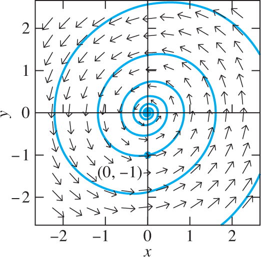
FIGURE 7.1.7.
Direction field and solution curve for the system of Example 7.

FIGURE 7.1.8.
x- and y-solution curves for the initial value problem of Example 7.
When we study linear systems in subsequent sections, we will learn why the superficially similar systems in Examples 5 through 7 have the markedly different trajectories shown in Figs. 7.1.4, 7.1.6, and 7.1.7.
Linear Systems
In addition to practical advantages for numerical computation, the general theory of systems and systematic solution techniques are more easily and more concisely described for first-order systems than for higher-order systems. For instance, consider a linear first-order system of the form
We say that this system is homogeneous if the functions are all identically zero; otherwise, it is nonhomogeneous. Thus the linear system in (5) is homogeneous, whereas the linear system in (11) is nonhomogeneous. The system in (10) is nonlinear because the right-hand side of the second equation is not a linear function of the dependent variables and .
A solution of the system in (20) is an n-tuple of functions that (on some interval) identically satisfy each of the equations in (20). We will see that the general theory of a system of n linear first-order equations shares many similarities with the general theory of a single nth-order linear differential equation. Theorem 1 (proved in Appendix A) is analogous to Theorem 2 of Section 5.2. It tells us that if the coefficient functions and in (20) are continuous, then the system has a unique solution satisfying given initial conditions.
Thus n initial conditions are needed to determine a solution of a system of n linear first-order equations, and we therefore expect a general solution of such a system to involve n arbitrary constants. For instance, we saw in Example 4 that the second-order linear system
which describes the position functions x(t) and y(t) of Example 1, is equivalent to the system of four first-order linear equations in (11). Hence four initial conditions would be needed to determine the subsequent motions of the two masses in Example 1. Typical initial values would be the initial positions x(0) and y(0) and the initial velocities and On the other hand, we found that the amounts x(t) and y(t) of salt in the two tanks of Example 2 are described by the system
of two first-order linear equations. Hence the two initial values x(0) and y(0) should suffice to determine the solution. Given a higher-order system, we often must transform it into an equivalent first-order system to discover how many initial conditions are needed to determine a unique solution. Theorem 1 tells us that the number of such conditions is precisely the same as the number of equations in the equivalent first-order system.
7.1 Problems
In Problems 1 through 10, transform the given differential equation or system into an equivalent system of first-order differential equations.
Use the method of Examples 5, 6, and 7 to find general solutions of the systems in Problems 11 through 20. If initial conditions are given, find the corresponding particular solution. For each problem, use a computer system or graphing calculator to construct a direction field and typical solution curves for the given system.
Calculate to show that the trajectories of the system of Problem 11 are circles.
Calculate to show that the trajectories of the system of Problem 12 are hyperbolas.
Beginning with the general solution of the system of Problem 13, calculate to show that the trajectories are circles.
Show similarly that the trajectories of the system of Problem 15 are ellipses with equations of the form .
First solve Eqs. (16) and (17) for and in terms of x(t), y(t), and the constants A and B. Then substitute the results in to show that the trajectories of the system in Example 6 satisfy an equation of the form
Then show that yields the straight lines and that are visible in Fig. 7.1.6.
Dual mass-spring system Derive the equations
for the displacements (from equilibrium) of the two masses shown in Fig. 7.1.9.

FIGURE 7.1.9.
The system of Problem 24.
Oscillating particles Two particles each of mass m are attached to a string under (constant) tension T, as indicated in Fig. 7.1.10. Assume that the particles oscillate vertically (that is, parallel to the y-axis) with amplitudes so small that the sines of the angles shown are accurately approximated by their tangents. Show that the displacements and satisfy the equations
where .

FIGURE 7.1.10.
The mechanical system of Problem 25.
Fermentation vats Three 100-gal fermentation vats are connected as indicated in Fig. 7.1.11, and the mixtures in each tank are kept uniform by stirring. Denote by the amount (in pounds) of alcohol in tank at time t (). Suppose that the mixture circulates between the tanks at the rate of 10 gal/min. Derive the equations

FIGURE 7.1.11.
The fermentation tanks of Problem 26.
A particle of mass m moves in the plane with coordinates (x(t), y(t)) under the influence of a force that is directed toward the origin and has magnitude —an inverse-square central force field. Show that
where .
Suppose that a projectile of mass m moves in a vertical plane in the atmosphere near the surface of the earth under the influence of two forces: a downward gravitational force of magnitude mg, and a resistive force that is directed opposite to the velocity vector v and has magnitude (where is the speed of the projectile; see Fig. 7.1.12). Show that the equations of motion of the projectile are
where .

FIGURE 7.1.12.
The trajectory of the projectile of Problem 28.
Suppose that a particle with mass m and electrical charge q moves in the xy-plane under the influence of the magnetic field (thus a uniform field parallel to the z-axis), so the force on the particle is if its velocity is v. Show that the equations of motion of the particle are
7.1 Application Gravitation and Kepler’s Laws of Planetary Motion
Around the turn of the seventeenth century, Johannes Kepler analyzed a lifetime of planetary observations by the astronomer Tycho Brahe. Kepler concluded that the motion of the planets around the sun is described by the following three propositions, now known as Kepler’s laws of planetary motion:
The orbit of each planet is an ellipse with the sun at one focus.
The radius vector from the sun to each planet sweeps out area at a constant rate.
The square of the planet’s period of revolution is proportional to the cube of the major semiaxis of its elliptical orbit.
In his Principia Mathematica (1687) Isaac Newton deduced the inverse square law of gravitation from Kepler’s laws. In this application we lead you (in the opposite direction) through a derivation of Kepler’s first two laws from Newton’s law of gravitation. Newton’s explanation of planetary motion in terms of gravitation is a landmark of scientific and intellectual history.
Assume that the sun is located at the origin in the plane of motion of a planet, and write the position vector of the planet in the form
where and denote the unit vectors in the positive x- and y-directions. Then the inverse-square law of gravitation implies (Problem 27) that the acceleration vector of the planet is given by
where is the distance from the sun to the planet. If the polar coordinates of the planet at time t are then the radial and transverse unit vectors shown in Fig. 7.1.13 are given by

FIGURE 7.1.13.
The radial and transverse unit vectors and
The radial unit vector (when located at the planet’s position) always points directly away from the origin, so and the transverse unit vector is obtained from by a counterclockwise rotation.
Step 1: Differentiate the equations in (3) componentwise to show that
Step 2: Use the equations in (4) to differentiate the planet’s position vector and thereby show that its velocity vector is given by
Step 3: Differentiate again to show that the planet’s acceleration vector is given by
Step 4: The radial and transverse components on the right-hand sides in Eqs. (2) and (6) must agree. Equating the transverse components—that is, the coefficients of —we get
so it follows that
where h is a constant. Because the polar-coordinate area element—for computation of the area A(t) in Fig. 7.1.14—is given by Eq. (8) implies that the derivative is constant, which is a statement of Kepler’s second law.

FIGURE 7.1.14.
Area swept out by the radius vector.
Step 5: Equate radial components in (2) and (6), and then use the result in (8) to show that the planet’s radial coordinate function r(t) satisfies the second-order differential equation
Step 6: Although the differential equation in (9) is nonlinear, it can be transformed to a linear equation by means of a simple substitution. For this purpose, assume that the orbit can be written in the polar-coordinate form and first use the chain rule and Eq. (8) to show that if then
Differentiate again, to deduce from Eq. (9) that the function satisfies the second-order equation
Step 7: Show that the general solution of Eq. (10) is
Step 8: Finally, deduce from Eq. (11) that is given by
with and The polar-coordinate graph of Eq. (12) is a conic section of eccentricity e—an ellipse if a parabola if and a hyperbola if —with focus at the origin. Planetary with perihelion distance and aphelion distance orbits are bounded and therefore are ellipses, with eccentricity As indicated in Fig. 7.1.15, the major axis of the ellipse lies along the radial line .

FIGURE 7.1.15.
The elliptical orbit
with perihelion distance
and aphelion distance
.
Step 9: Plot some typical elliptical orbits—as described by (12)—having different eccentricities, sizes, and orientations. In rectangular coordinates you can write
to plot an elliptical orbit with eccentricity e, semilatus rectum L (Fig. 7.1.15), and rotation angle The eccentricity of the earth’s orbit is so close to zero that the orbit looks nearly circular (though with the sun off center), and the eccentricities of the other planetary orbits range from 0.0068 for Venus and 0.0933 for Mars to 0.2056 for Mercury (and 0.2486 for Pluto, no longer classified a planet). But many comets have highly eccentric orbits—Halley’s comet has (Fig.7.1.16).

FIGURE 7.1.16.
The shape of the orbit of Halley’s comet.