Search in book...
Toggle Font Controls
Create new playlist

Name your new playlist

Playlist description (optional)
Sign In

Email address

Password

Forgot Password?

or

Continue with Facebook

Continue with Google
Sign Up

Full Name

Email address

Confirm Email Address

Password

or

Continue with Facebook

Continue with Google

10.5 Periodic and Piecewise Continuous Input Functions

Mathematical models of mechanical or electrical systems often involve functions with discontinuities corresponding to external forces that are turned abruptly on or off. One such simple on–off function is the unit step function that we introduced in Section 10.1. Recall that the unit step function at t=a $t = a$ is defined by

u a (t) = u (t - a) = {01 if t < a, if t ≧ a .

$u_{a} (t) = u (t - a) = {\begin{array}{l} 0 & if t < a, \\ 1 & if t ≧ a . \end{array}$ (1)

The notation ua(t) $u_{a} (t)$ indicates succinctly where the unit upward step in value takes place (Fig. 10.5.1), whereas u(t−a) $u (t - a)$ connotes the sometimes useful idea of a “time delay” a before the step is made.

In Example 8 of Section 10.1 we saw that if a≧0, $a ≧ 0,$ then

FIGURE 10.5.1.

The graph of the unit step function at t=a. $t = a .$

L {u (t - a)} = e - a s s .

$L {u (t - a)} = \frac{e^{- a s}}{s} .$ (2)

Because L{u(t)}=1/s, $L {u (t)} = 1 / s,$ Eq. (2) implies that multiplication of the transform of u(t) by e−as $e^{- a s}$ corresponds to the translation t→t−a $t \to t - a$ in the original independent variable. Theorem 1 tells us that this fact, when properly interpreted, is a general property of the Laplace transformation.

Note that

u (t - a) f (t - a) = {0 f (t - a) if t < a, if t ≧ a .

$u (t - a) f (t - a) = {\begin{array}{l} 0 & if t < a, \\ f (t - a) & if t ≧ a . \end{array}$ (4)

Thus Theorem 1 implies that L−1{e−asF(s)} $L^{- 1} {e^{- a s} F (s)}$ is the function whose graph for t≧a $t ≧ a$ is the translation by a units to the right of the graph of f(t) for t≧0. $t ≧ 0 .$ Note that the part (if any) of the graph of f(t) to the left of t=0 $t = 0$ is “cut off” and is not translated (Fig. 10.5.2). In some applications the function f(t) describes an incoming signal that starts arriving at time t=0. $t = 0 .$ Then u(t−a)f(t−a) $u (t - a) f (t - a)$ denotes a signal of the same “shape” but with a time delay of a, so it does not start arriving until time t=a $t = a$ .

FIGURE 10.5.2.

Translation of f(t) a units to the right.

Proof of Theorem 1:

From the definition of L{f(t)}, $L {f (t)},$ we get

e - a s F (s) = e - a s \int \infty 0 e - s τ f (τ) d τ = \int \infty 0 e - s (τ + a) f (τ) d τ .

$e^{- a s} F (s) = e^{- a s} \int_{0}^{\infty} e^{- s τ} f (τ) d τ = \int_{0}^{\infty} e^{- s (τ + a)} f (τ) d τ .$

The substitution t=τ+a $t = τ + a$ then yields

e - a s F (s) = \int \infty a e - s t f (t - a) d t .

$e^{- a s} F (s) = \int_{a}^{\infty} e^{- s t} f (t - a) d t .$

From Eq. (4) we see that this is the same as

e - a s F (s) = \int \infty 0 e - s t u (t - a) f (t - a) d t = L {u (t - a) f (t - a)},

$e^{- a s} F (s) = \int_{0}^{\infty} e^{- s t} u (t - a) f (t - a) d t = L {u (t - a) f (t - a)},$

because u(t−a)f(t−a)=0 $u (t - a) f (t - a) = 0$ for t<a. $t < a .$ This completes the proof of Theorem 1.

Example 1

With f(t)=12t2, $f (t) = \frac{1}{2} t^{2},$ Theorem 1 gives

L - 1 {e - a s s 3} = u (t - a) 1 2 (t - a) 2 = {0 1 2 (t - a) 2 if t < a, if t ≧ a (Fig . 10.5.3) .

$\begin{array}{l} L^{- 1} {\frac{e^{- a s}}{s^{3}}} = u (t - a) \frac{1}{2} {(t - a)}^{2} = {\begin{array}{l} 0 & if t < a, \\ \frac{1}{2} {(t - a)}^{2} & if t ≧ a \end{array} & (Fig . 10.5.3) . \end{array}$

Example 2

Find L{g(t)} $L {g (t)}$ if

g (t) = {0 t 2 if t < 3, if t ≧ 3 (Fig . 10.5.4) .

$\begin{array}{l} g (t) = {\begin{array}{l} 0 & if t < 3, \\ t^{2} & if t ≧ 3 \end{array} & (Fig . 10.5.4) . \end{array}$

Solution

Before applying Theorem 1, we must first write g(t) in the form u(t−3)f(t−3). $u (t - 3) f (t - 3) .$ The function f(t) whose translation 3 units to the right agrees (for t≧3 $t ≧ 3$ ) with g(t)=t2 $g (t) = t^{2}$ is f(t)=(t+3)2 $f (t) = {(t + 3)}^{2}$ because f(t−3)=t2. $f (t - 3) = t^{2} .$ But then

F (s) = L {t 2 + 6 t + 9} = 2 s 3 + 6 s 2 + 9 s,

$F (s) = L {t^{2} + 6 t + 9} = \frac{2}{s^{3}} + \frac{6}{s^{2}} + \frac{9}{s},$

so now Theorem 1 yields

L {g (t)} = L {u (t - 3) f (t - 3)} = e - 3 s F (s) = e - 3 s (2 s 3 + 6 s 2 + 9 s) .

$L {g (t)} = L {u (t - 3) f (t - 3)} = e^{- 3 s} F (s) = e^{- 3 s} (\frac{2}{s^{3}} + \frac{6}{s^{2}} + \frac{9}{s}) .$

FIGURE 10.5.3.

The graph of the inverse transform of Example 1.

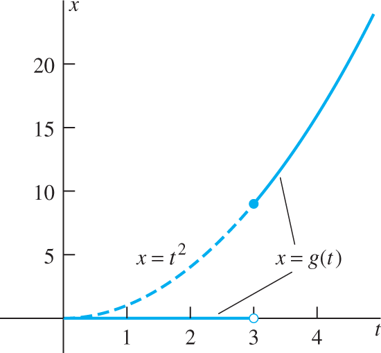
FIGURE 10.5.4.

The graph of the function `g`(`t`) of Example 2.

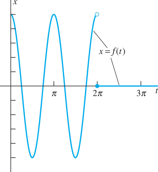
FIGURE 10.5.5.

The function `f`(`t`) of Examples 3 and 4.

Example 3

Find L{f(t)} $L {f (t)}$ if

f (t) = {cos 2 t 0 if 0 ≦ t < 2 π, if t ≧ 2 π (Fig .10 .5 .5) .

$f (t) = {\begin{array}{l} \cos 2 t & if 0 ≦ t < 2 π, \\ 0 & if t ≧ 2 π \end{array} (Fig .10 .5 .5) .$

Solution

We note first that

f (t) = [1 - u (t - 2 π)] cos 2 t = cos 2 t - u (t - 2 π) cos 2 (t - 2 π)

$f (t) = [1 - u (t - 2 π)] \cos 2 t = \cos 2 t - u (t - 2 π) \cos 2 (t - 2 π)$

because of the periodicity of the cosine function. Hence Theorem 1 gives

L {f (t)} = L {cos 2 t} - e - 2 π s L {cos 2 t} = s ( 1 - e - 2 π s ) s 2 + 4 .

$L {f (t)} = L {\cos 2 t} - e^{- 2 π s} L {\cos 2 t} = \frac{s (1 - e^{- 2 π s})}{s^{2} + 4} .$

Example 4

Discontinuous forcing A mass that weighs 32 lb (mass m=1 $m = 1$ slug) is attached to the free end of a long light spring that is stretched 1 ft by a force of 4 lb (k=4 $k = 4$ lb/ft). The mass is initially at rest in its equilibrium position. Beginning at time t=0 $t = 0$ (seconds), an external force F(t)=cos 2t $F (t) = \cos 2 t$ is applied to the mass, but at time t=2π $t = 2 π$ this force is turned off (abruptly discontinued) and the mass is allowed to continue its motion unimpeded. Find the resulting position function x(t) of the mass.

Solution

We need to solve the initial value problem

x'' + 4 x = f (t); x (0) = x' (0) = 0,

$x^{″} + 4 x = f (t); x (0) = x^{′} (0) = 0,$

where f(t) is the function of Example 3. The transformed equation is

(s 2 + 4) X (s) = F (s) = s ( 1 - e - 2 π s ) s 2 + 4,

$(s^{2} + 4) X (s) = F (s) = \frac{s (1 - e^{- 2 π s})}{s^{2} + 4},$

X (s) = s ( s 2 + 4 ) 2 - e - 2 π s s ( s 2 + 4 ) 2 .

$X (s) = \frac{s}{{(s^{2} + 4)}^{2}} - e^{- 2 π s} \frac{s}{{(s^{2} + 4)}^{2}} .$

Because

L - 1 {s ( s 2 + 4 ) 2} = 1 4 t sin 2 t

$L^{- 1} {\frac{s}{{(s^{2} + 4)}^{2}}} = \frac{1}{4} t \sin 2 t$

by Eq. (16) of Section 10.3, it follows from Theorem 1 that

x (t) = = 1 4 t sin 2 t - u (t - 2 π) \cdot 1 4 (t - 2 π) sin 2 (t - 2 π) 1 4 [t - u (t - 2 π) \cdot (t - 2 π)] sin 2 t .

$\begin{array}{rcl} x (t) & = & \frac{1}{4} t \sin 2 t - u (t - 2 π) \cdot \frac{1}{4} (t - 2 π) \sin 2 (t - 2 π) \\ = & \frac{1}{4} [t - u (t - 2 π) \cdot (t - 2 π)] \sin 2 t . \end{array}$

If we separate the cases t<2π $t < 2 π$ and t≧2π, $t ≧ 2 π,$ we find that the position function may be written in the form

x (t) = {1 4 t sin 2 t 1 2 π sin 2 t if t < 2 π, if t ≧ 2 π .

$x (t) = {\begin{array}{l} \frac{1}{4} t \sin 2 t & if t < 2 π, \\ \frac{1}{2} π \sin 2 t & if t ≧ 2 π . \end{array}$

As indicated by the graph of x(t) shown in Fig. 10.5.6, the mass oscillates with circular frequency ω=2 $ω = 2$ and with linearly increasing amplitude until the force is removed at time t=2π. $t = 2 π .$ Thereafter, the mass continues to oscillate with the same frequency but with constant amplitude π/2. $π / 2 .$ The force F(t)=cos 2t $F (t) = \cos 2 t$ would produce pure resonance if continued indefinitely, but we see that its effect ceases immediately at the moment it is turned off.

FIGURE 10.5.6.

The graph of the function `x`(`t`) of Example 4.

If we were to attack Example 4 with the methods of Chapter 5, we would need to solve one problem for the interval 0≦t<2π $0 ≦ t < 2 π$ and then solve a new problem with different initial conditions for the interval t≧2π. $t ≧ 2 π .$ In such a situation the Laplace transform method enjoys the distinct advantage of not requiring the solution of different problems on different intervals.

Transforms of Periodic Functions

Periodic forcing functions in practical mechanical or electrical systems often are more complicated than pure sines or cosines. The nonconstant function f(t) defined for t≧0 $t ≧ 0$ is said to be periodic if there is a number p>0 $p > 0$ such that

f (t + p) = f (t)

$f (t + p) = f (t)$ (5)

for all t≧0. $t ≧ 0 .$ The least positive value of p (if any) for which Eq. (11) holds is called the period of f. Such a function is shown in Fig. 10.5.7. Theorem 2 simplifies the computation of theLaplace transform of a periodic function.

FIGURE 10.5.7.

The graph of a function with period `p`.

Proof:

The definition of the Laplace transform gives

F (s) = \int \infty 0 e - s t f (t) d t = \sum n = 0 \infty \int (n + 1) p n p e - s t f (t) d t .

$F (s) = \int_{0}^{\infty} e^{- s t} f (t) d t = \sum_{n = 0}^{\infty} \int_{n p}^{(n + 1) p} e^{- s t} f (t) d t .$

The substitution t=τ+np $t = τ + n p$ in the nth integral following the summation sign yields

\int (n + 1) p n p e - s t f (t) d t = \int p 0 e - s (τ + n p) f (τ + n p) d τ = e - n p s \int p 0 e - s τ f (τ) d τ

$\int_{n p}^{(n + 1) p} e^{- s t} f (t) d t = \int_{0}^{p} e^{- s (τ + n p)} f (τ + n p) d τ = e^{- n p s} \int_{0}^{p} e^{- s τ} f (τ) d τ$

because f(τ+np)=f(τ) $f (τ + n p) = f (τ)$ by periodicity. Thus

F (s) = = \sum n = 0 \infty (e - n p s \int p 0 e - s τ f (τ) d τ) (1 + e - p s + e - 2 p s + \dots) \int p 0 e - s τ f (τ) d τ .

$\begin{array}{rcl} F (s) & = & \sum_{n = 0}^{\infty} (e^{- n p s} \int_{0}^{p} e^{- s τ} f (τ) d τ) \\ = & (1 + e^{- p s} + e^{- 2 p s} + \dots) \int_{0}^{p} e^{- s τ} f (τ) d τ . \end{array}$

Consequently,

F (s) = 1 1 - e - p s \int p 0 e - s τ f (τ) d τ .

$F (s) = \frac{1}{1 - e^{- p s}} \int_{0}^{p} e^{- s τ} f (τ) d τ .$

We use the geometric series

1 1 - x = 1 + x + x 2 + x 3 + \dots,

$\frac{1}{1 - x} = 1 + x + x^{2} + x^{3} + \dots,$

with x=e−ps<1 $x = e^{- p s} < 1$ (for s>0 $s > 0$ ) to sum the series in the final step. Thus we have derived Eq. (6).

The principal advantage of Theorem 2 is that it enables us to find the Laplace transform of a periodic function without the necessity of an explicit evaluation of an improper integral.

Example 5

Figure 10.5.8 shows the graph of the square wave function f(t)=(−1)〚t/a〛 $f (t) = {(- 1)}^{〚 t / a 〛}$ of period p=2a; 〚x〛 $p = 2 a; 〚 x 〛$ denotes the greatest integer not exceeding x. By Theorem 2 theLaplace transform of f(t) is

F (s) = = = = 1 1 - e - 2 a s \int 2 a 0 e - s t f (t) d t 1 1 - e - 2 a s (\int a 0 e - s t d t + \int 2 a a (- 1) e - s t d t) 1 1 - e - 2 a s ([- 1 s e - s t] a 0 - [- 1 s e - s t] 2 a a) ( 1 - e - a s ) 2 s ( 1 - e - 2 a s ) = 1 - e - a s s ( 1 + e - a s ) .

$\begin{array}{rcl} F (s) & = & \frac{1}{1 - e^{- 2 a s}} \int_{0}^{2 a} e^{- s t} f (t) d t \\ = & \frac{1}{1 - e^{- 2 a s}} (\int_{0}^{a} e^{- s t} d t + \int_{a}^{2 a} (- 1) e^{- s t} d t) \\ = & \frac{1}{1 - e^{- 2 a s}} ({[- \frac{1}{s} e^{- s t}]}_{0}^{a} - {[- \frac{1}{s} e^{- s t}]}_{a}^{2 a}) \\ = & \frac{{(1 - e^{- a s})}^{2}}{s (1 - e^{- 2 a s})} = \frac{1 - e^{- a s}}{s (1 + e^{- a s})} . \end{array}$

Therefore,

F (s) = 1 - e - a s s ( 1 + e - a s )

$F (s) = \frac{1 - e^{- a s}}{s (1 + e^{- a s})}$ (7a)

= e a s / 2 - e - a s / 2 s ( e a s / 2 + e - a s / 2 ) = 1 s tanh a s 2 .

$= \frac{e^{a s / 2} - e^{- a s / 2}}{s (e^{a s / 2} + e^{- a s / 2})} = \frac{1}{s} \tanh \frac{a s}{2} .$ (7b)

FIGURE 10.5.8.

The graph of the square wave function of Example 5.

Example 6

Figure 10.5.9 shows the graph of a triangular wave function g(t) of period p=2a. $p = 2 a .$ Becausethe derivative g'(t) $g^{′} (t)$ is thesquare wave function of Example 6, it follows from the formula in (7b) and Theorem 2 of Section 10.2 that the transform of this triangular wavefunction is

G (s) = F ( s ) s = 1 s 2 tanh a s 2 .

$G (s) = \frac{F (s)}{s} = \frac{1}{s^{2}} \tanh \frac{a s}{2} .$ (8)

FIGURE 10.5.9.

The graph of the triangular wave function of Example 6.

Example 7

Square wave forcing Consider a mass–spring–dashpot system with m=1, c=4, $m = 1, c = 4,$ and k=20 $k = 20$ in appropriate units. Suppose that the system is initially at rest at equilibrium (x(0)=x'(0)=0) $(x (0) = x^{′} (0) = 0)$ and that the mass is acted on beginning at time t=0 $t = 0$ by the external force f(t) whose graph is shown in Fig. 10.5.10: the square wave with amplitude 20 and period 2π. $2 π .$ Find the position function f(t).

Solution

The initial value problem is

x'' + 4 x' + 20 x = f (t); x (0) = x' (0) = 0.

$x^{″} + 4 x^{′} + 20 x = f (t); x (0) = x^{′} (0) = 0.$

The transformed equation is

s 2 X (s) + 4 s X (s) + 20 X (s) = F (s) .

$s^{2} X (s) + 4 s X (s) + 20 X (s) = F (s) .$ (9)

FIGURE 10.5.10.

The graph of the external force function of Example 7.

From Example 5 with a=π $a = π$ we see that the transform of f(t) is

F (s) = = = 20 s \cdot 1 - e - π s 1 + e - π s 20 s (1 - e - π s) (1 - e - π s + e - 2 π s - e - 3 π s + \dots) 20 s (1 - 2 e - π s + 2 e - 2 π s - 2 e - 3 π s + \dots),

$\begin{array}{rcl} F (s) & = & \frac{20}{s} \cdot \frac{1 - e^{- π s}}{1 + e^{- π s}} \\ = & \frac{20}{s} (1 - e^{- π s}) (1 - e^{- π s} + e^{- 2 π s} - e^{- 3 π s} + \dots) \\ = & \frac{20}{s} (1 - 2 e^{- π s} + 2 e^{- 2 π s} - 2 e^{- 3 π s} + \dots), \end{array}$

so that

F (s) = 20 s + 40 s \sum n = 1 \infty (- 1) n e - n π s .

$F (s) = \frac{20}{s} + \frac{40}{s} \sum_{n = 1}^{\infty} {(- 1)}^{n} e^{- n π s} .$ (10)

Substitution of Eq. (10) in Eq. (9) yields

X (s) = = F ( s ) s 2 + 4 s + 20 20 s [ ( s + 2 ) 2 + 16 ] + 2 \sum n = 1 \infty (- 1) n 20 e - n π s s [ ( s + 2 ) 2 + 16 .

$\begin{array}{rcl} X (s) & = & \frac{F (s)}{s^{2} + 4 s + 20} \\ = & \frac{20}{s [{(s + 2)}^{2} + 16]} + 2 \sum_{n = 1}^{\infty} {(- 1)}^{n} \frac{20 e^{- n π s}}{s [{(s + 2)}^{2} + 16} . \end{array}$ (11)

From the transform in Eq. (8) of Section 10.3, we get

L - 1 {20 ( s + 2 ) 2 + 16} = 5 e - 2 t sin 4 t,

$L^{- 1} {\frac{20}{{(s + 2)}^{2} + 16}} = 5 e^{- 2 t} \sin 4 t,$

so by Theorem 2 of Section 10.2 we have

g (t) = L - 1 {20 s [ ( s + 2 ) 2 + 16 ]} = \int t 0 5 e - 2 τ sin 4 τ d τ .

$g (t) = L^{- 1} {\frac{20}{s [{(s + 2)}^{2} + 16]}} = \int_{0}^{t} 5 e^{- 2 τ} \sin 4 τ d τ .$

Using a tabulated formula for ∫eat sin bt dt, $\int e^{a t} \sin b t d t,$ we get

g (t) = 1 - e - 2 t (cos 4 t + 1 2 sin 4 t) = 1 - h (t),

$g (t) = 1 - e^{- 2 t} (\cos 4 t + \frac{1}{2} \sin 4 t) = 1 - h (t),$ (12)

where

h (t) = e - 2 t (cos 4 t + 1 2 sin 4 t) .

$h (t) = e^{- 2 t} (\cos 4 t + \frac{1}{2} \sin 4 t) .$ (13)

Now we apply Theorem 1 to find the inverse transform of the right-hand term in Eq. (11). The result is

x (t) = g (t) + 2 \sum n = 1 \infty (- 1) n u (t - n π) g (t - n π),

$x (t) = g (t) + 2 \sum_{n = 1}^{\infty} {(- 1)}^{n} u (t - n π) g (t - n π),$ (14)

and we note that for any fixed value of t the sum in Eq. (14) is finite. Moreover,

g (t - n π) = = 1 - e - 2 (t - n π) [cos 4 (t - n π) + 1 2 sin 4 (t - n π)] 1 - e 2 n π e - 2 t (cos 4 t + 1 2 sin 4 t) .

$\begin{array}{rcl} g (t - n π) & = & 1 - e^{- 2 (t - n π)} [\cos 4 (t - n π) + \frac{1}{2} \sin 4 (t - n π)] \\ = & 1 - e^{2 n π} e^{- 2 t} (\cos 4 t + \frac{1}{2} \sin 4 t) . \end{array}$

Therefore,

g (t - n π) = 1 - e 2 n π h (t) .

$g (t - n π) = 1 - e^{2 n π} h (t) .$ (15)

Hence if 0<t<π, $0 < t < π,$ then

x (t) = 1 - h (t) .

$x (t) = 1 - h (t) .$

If π<t<2π, $π < t < 2 π,$ then

x (t) = [1 - h (t)] - 2 [1 - e 2 π h (t)] = - 1 + h (t) - 2 h (t) [1 - e 2 π] .

$x (t) = [1 - h (t)] - 2 [1 - e^{2 π} h (t)] = - 1 + h (t) - 2 h (t) [1 - e^{2 π}] .$

If 2π<t<3π, $2 π < t < 3 π,$ then

x (t) = = [1 - h (t)] - 2 [1 - e 2 π h (t)] + 2 [1 - e 4 π h (t)] 1 + h (t) - 2 h (t) [1 - e 2 π + e 4 π] .

$\begin{array}{rcl} x (t) & = & [1 - h (t)] - 2 [1 - e^{2 π} h (t)] + 2 [1 - e^{4 π} h (t)] \\ = & 1 + h (t) - 2 h (t) [1 - e^{2 π} + e^{4 π}] . \end{array}$

The general expression for nπ<t<(n+1)π $n π < t < (n + 1) π$ is

x (t) = = h (t) + (- 1) n - 2 h (t) [1 - e 2 π + \dots + (- 1) n e 2 n π] h (t) + (- 1) n - 2 h (t) 1 + ( - 1 ) n e 2 ( n + 1 ) π 1 + e 2 π,

$\begin{array}{rcl} x (t) & = & h (t) + {(- 1)}^{n} - 2 h (t) [1 - e^{2 π} + \dots + {(- 1)}^{n} e^{2 n π}] \\ = & h (t) + {(- 1)}^{n} - 2 h (t) \frac{1 + {(- 1)}^{n} e^{2 (n + 1) π}}{1 + e^{2 π}}, \end{array}$ (16)

which we obtained with the aid of the familiar formula for the sum of a finite geometric progression. A rearrangement of Eq. (16) finally gives, with the aid of Eq. (13),

x (t) = e 2 π - 1 e 2 π + 1 e - 2 t (cos 4 t + 1 2 sin 4 t) + (- 1) n - 2 \cdot ( - 1 ) n e 2 π e 2 π + 1 e - 2 (t - n π) (cos 4 t + 1 2 sin 4 t)

$\begin{array}{rcl} x (t) & = & \frac{e^{2 π} - 1}{e^{2 π} + 1} e^{- 2 t} (\cos 4 t + \frac{1}{2} \sin 4 t) + {(- 1)}^{n} \\ - \frac{2 \cdot {(- 1)}^{n} e^{2 π}}{e^{2 π} + 1} e^{- 2 (t - n π)} (\cos 4 t + \frac{1}{2} \sin 4 t) \end{array}$ (17)

for nπ<t<(n+1)π. $n π < t < (n + 1) π .$ The first term in Eq. (17) is the transient solution

x tr (t) \approx (0.9963) e - 2 t (cos 4 t + 1 2 sin 4 t) \approx (1.1139) e - 2 t cos (4 t - 0.4636) .

$x_{tr} (t) \approx (0.9963) e^{- 2 t} (\cos 4 t + \frac{1}{2} \sin 4 t) \approx (1.1139) e^{- 2 t} \cos (4 t - 0.4636) .$ (18)

The last two terms in Eq. (17) give the steady periodic solution xsp. $x_{sp} .$ To investigate it, we write τ=t−nπ $τ = t - n π$ for t in the interval nπ<t<(n+1)π. $n π < t < (n + 1) π .$ Then

x sp (t) = \approx (- 1) n [1 - 2 e 2 π e 2 π + 1 e - 2 τ (cos 4 τ + 1 2 sin 4 τ)] (- 1) n [1 - (2.2319) e - 2 τ cos (4 τ - 0.4636)] .

$\begin{array}{rcl} x_{sp} (t) & = & {(- 1)}^{n} [1 - \frac{2 e^{2 π}}{e^{2 π} + 1} e^{- 2 τ} (\cos 4 τ + \frac{1}{2} \sin 4 τ)] \\ \approx & {(- 1)}^{n} [1 - (2.2319) e^{- 2 τ} \cos (4 τ - 0.4636)] . \end{array}$ (19)

Figure 10.5.11 shows the graph of xsp(t). $x_{sp} (t) .$ Its most interesting feature is the appearance of periodically damped oscillations with a frequency four times that of the imposed force f(t).

FIGURE 10.5.11.

The graph of the steady periodic solution for Example 7; note the “periodically damped” oscillations with frequency four times that of the imposed force.

10.5 Problems

Find the inverse Laplace transform f(t) of each function given in Problems 1 through 10. Then sketch the graph of f.

F(s)=e−3ss2 $F (s) = \frac{e^{- 3 s}}{s^{2}}$
F(s)=e−s−e−3ss2 $F (s) = \frac{e^{- s} - e^{- 3 s}}{s^{2}}$
F(s)=e−ss+2 $F (s) = \frac{e^{- s}}{s + 2}$
F(s)=e−s−e2−2ss−1 $F (s) = \frac{e^{- s} - e^{2 - 2 s}}{s - 1}$
F(s)=e−πss2+1 $F (s) = \frac{e^{- π s}}{s^{2} + 1}$
F(s)=se−ss2+π2 $F (s) = \frac{s e^{- s}}{s^{2} + π^{2}}$
F(s)=1−e−2πss2+1 $F (s) = \frac{1 - e^{- 2 π s}}{s^{2} + 1}$
F(s)=s(1−e−2s)s2+π2 $F (s) = \frac{s (1 - e^{- 2 s})}{s^{2} + π^{2}}$
F(s)=s(1+e−3s)s2+π2 $F (s) = \frac{s (1 + e^{- 3 s})}{s^{2} + π^{2}}$
F(s)=2s(e−πs−e−2πs)s2+4 $F (s) = \frac{2 s (e^{- π s} - e^{- 2 π s})}{s^{2} + 4}$

Find the Laplace transforms of the functions given in Problems 11 through 22.

f(t)=2 $f (t) = 2$ if 0≦t<3; $0 ≦ t < 3;$ f(t)=0 $f (t) = 0$ if t≧3 $t ≧ 3$
f(t)=1 $f (t) = 1$ if 1≦t≦4; $1 ≦ t ≦ 4;$ f(t)=0 $f (t) = 0$ if t<1 $t < 1$ or if t>4 $t > 4$
f(t)=sin t $f (t) = \sin t$ if 0≦t≦2π; $0 ≦ t ≦ 2 π;$ f(t)=0 $f (t) = 0$ if t>2π $t > 2 π$
f(t)=cos πt $f (t) = \cos π t$ if 0≦t≦2; $0 ≦ t ≦ 2;$ f(t)=0 $f (t) = 0$ if t>2 $t > 2$
f(t)=sin t $f (t) = \sin t$ if 0≦t≦3π; $0 ≦ t ≦ 3 π;$ f(t)=0 $f (t) = 0$ if t>3π $t > 3 π$
f(t)=sin 2t $f (t) = \sin 2 t$ if π≦t≦2π; $π ≦ t ≦ 2 π;$ f(t)=0 $f (t) = 0$ if t<π $t < π$ or if t>2π $t > 2 π$
f(t)=sin πt $f (t) = \sin π t$ if 2≦t≦3; $2 ≦ t ≦ 3;$ f(t)=0 $f (t) = 0$ if t<2 $t < 2$ or if t>3 $t > 3$
f(t)=cos12πt $f (t) = \cos \frac{1}{2} π t$ if 3≦t≦5 $3 ≦ t ≦ 5$ ; f(t)=0 $f (t) = 0$ if t<3 $t < 3$ or if t>5 $t > 5$
f(t)=0 $f (t) = 0$ if t<1; $t < 1;$ f(t)=t $f (t) = t$ if t≧1 $t ≧ 1$
f(t)=t $f (t) = t$ if t≦1; $t ≦ 1;$ f(t)=1 $f (t) = 1$ if t>1 $t > 1$
f(t)=t $f (t) = t$ if t≦1; $t ≦ 1;$ f(t)=2−t $f (t) = 2 - t$ if 1≦t≦2; $1 ≦ t ≦ 2;$ f(t)=0 $f (t) = 0$ if t>2 $t > 2$
f(t)=t3 $f (t) = t^{3}$ if 1≦t≦2; $1 ≦ t ≦ 2;$ f(t)=0 $f (t) = 0$ if t<1 $t < 1$ or if t>2 $t > 2$
Apply Theorem 2 with p=1 $p = 1$ to verify that L{1}=1/s. $L {1} = 1 / s .$
Apply Theorem 2 to verify that L{cos kt}=s/(s2+k2) $L {\cos k t} = s / (s^{2} + k^{2})$ .
Apply Theorem 2 to show that the Laplace transform of the square wave function of Fig. 10.5.12 is

$L {f (t)} = 1 s ( 1 + e - a s ) .$ $L {f (t)} = \frac{1}{s (1 + e^{- a s})} .$

FIGURE 10.5.12.

The graph of the square wave function of Problem 25.
Apply Theorem 2 to show that the Laplace transform of the sawtooth function f(t) of Fig. 10.5.13 is

$F (s) = 1 a s 2 - e - a s s ( 1 - e - a s ) .$ $F (s) = \frac{1}{a s^{2}} - \frac{e^{- a s}}{s (1 - e^{- a s})} .$

FIGURE 10.5.13.

The graph of the sawtooth function of Problem 26.
Let g(t) be the staircase function of Fig. 10.5.14. Show that g(t)=(t/a)−f(t), $g (t) = (t / a) - f (t),$ where f is the sawtooth function of Fig. 10.5.14, and hence deduce that

$L {g (t)} = e - a s s ( 1 - e - a s ) .$ $L {g (t)} = \frac{e^{- a s}}{s (1 - e^{- a s})} .$

FIGURE 10.5.14.

The graph of the staircase function of Problem 27.
Suppose that f(t) is a periodic function of period 2a with f(t)=t $f (t) = t$ if 0≦t<a $0 ≦ t < a$ and f(t)=0 $f (t) = 0$ if a≦t<2a. $a ≦ t < 2 a .$ Find L{f(t)} $L {f (t)}$ .
Suppose that f(t) is the half-wave rectification of sin kt, $\sin k t,$ shown in Fig. 10.5.15. Show that

$L {f (t)} = k ( s 2 + k 2 ) ( 1 - e - π s / k ) .$ $L {f (t)} = \frac{k}{(s^{2} + k^{2}) (1 - e^{- π s / k})} .$

FIGURE 10.5.15.

The half-wave rectification of sin kt. $\sin k t .$
Let g(t)=u(t−π/k)f(t−π/k), $g (t) = u (t - π / k) f (t - π / k),$ where f(t) is the function of Problem 29 and k>0. $k > 0 .$ Note that h(t)=f(t)+g(t) $h (t) = f (t) + g (t)$ is the full-wave rectification of sin kt $\sin k t$ shown in Fig. 10.5.16. Hence deduce from Problem 29 that

$L {h (t)} = k s 2 + k 2 coth π s 2 k .$ $L {h (t)} = \frac{k}{s^{2} + k^{2}} \coth \frac{π s}{2 k} .$

FIGURE 10.5.16.

The full-wave rectification of sin kt. $\sin k t .$

Discontinuous Forcing

In Problems 31 through 35, the values of mass m, spring constant k, dashpot resistance c, and force f(t) are given for a mass–spring–dashpot system with external forcing function. Solve the initial value problem

m x'' + c x' + k x = f (t); x (0) = x' (0) = 0

$m x^{″} + c x^{′} + k x = f (t); x (0) = x^{′} (0) = 0$

and construct the graph of the position function x(t).

m=1, k=4, c=0; $m = 1, k = 4, c = 0;$ f(t)=1 $f (t) = 1$ if 0≦t<π, $0 ≦ t < π,$ f(t)=0 $f (t) = 0$ if t≧π $t ≧ π$
m=1, k=4, c=5; $m = 1, k = 4, c = 5;$ f(t)=1 $f (t) = 1$ if 0≦t<2, $0 ≦ t < 2,$ f(t)=0 $f (t) = 0$ if t≧2 $t ≧ 2$
m=1, k=9, c=0; $m = 1, k = 9, c = 0;$ f(t)=sin t $f (t) = \sin t$ if 0≦t≦2π, $0 ≦ t ≦ 2 π,$ f(t)=0 $f (t) = 0$ if t>2π $t > 2 π$
m=1, k=1, c=0; $m = 1, k = 1, c = 0;$ f(t)=t $f (t) = t$ if 0≦t<1, $0 ≦ t < 1,$ f(t)=0 $f (t) = 0$ if t≧1 $t ≧ 1$
m=1, k=4, c=4; $m = 1, k = 4, c = 4;$ f(t)=t $f (t) = t$ if 0≦t≦2, $0 ≦ t ≦ 2,$ f(t)=0 $f (t) = 0$ if t>2 $t > 2$

Transient and Steady Periodic Motions

In Problems 36 and 37, a mass–spring–dashpot system with external force f(t) is described. Under the assumption that x(0)=x'(0)=0, $x (0) = x^{′} (0) = 0,$ use the method of Example 7 to find the transient and steady periodic motions of the mass. Then construct the graph of the position function x(t). If you would like to check your graph using a numerical DE solver, it may be useful to note that the function

f (t) = A [2 u ((t - π) (t - 2 π) (t - 3 π) . (t - 4 π) (t - 5 π) (t - 6 π)) - 1]

$\begin{array}{l} f (t) = A [2 u ((t - π) (t - 2 π) (t - 3 π) . \\ (t - 4 π) (t - 5 π) (t - 6 π)) - 1] \end{array}$

has the value +A $+ A$ if 0<t<π, $0 < t < π,$ the value −A $- A$ if π<t<2π, $π < t < 2 π,$ and so forth, and hence agrees on the interval [0,6π] $[0, 6 π]$ with the square wave function that has amplitude A and period 2π. $2 π .$ (See also the definition of a square wave function interms of sawtooth and triangular wave functions in the application material for this section.)

m=1, k=4, c=0; $m = 1, k = 4, c = 0;$ f(t) is a square wave function with amplitude 4 and period 2π $2 π$ .
m=1, k=10, c=2; $m = 1, k = 10, c = 2;$ f(t) is a square wave function with amplitude 10 andperiod 2π $2 π$ .
Suppose the function x(t) satisfies the initial value problem

$m x'' + c x' + k x = F (t), x (a) = b 0, x' (a) = b 1$ $m x^{″} + c x^{′} + k x = F (t), x (a) = b_{0}, x^{′} (a) = b_{1}$

for t≧a $t ≧ a$ and x(t)=0 $x (t) = 0$ for t<a. $t < a .$ Then show that X(s)=L{x(t)} $X (s) = L {x (t)}$ satisfies the equation

$m (s 2 (e a s X) - s b 0 - b 1) + c (s (e a s X) - b 0) + k (e a s X) = L {F (t + a)} .$ $\begin{array}{l} m (s^{2} (e^{a s} X) - s b_{0} - b_{1}) + c (s (e^{a s} X) - b_{0}) + k (e^{a s} X) \\ = L {F (t + a)} . \end{array}$
This is an alternate approach to Example 7 that was suggested by Keng C. Wu of Lockheed Martin (Maritime Systems Sensors). Let x(t) denote the steady periodic solution of the given differential equation x′′+4x'+20x=F(t). $x^{″} + 4 x^{′} + 20 x = F (t) .$ Suppose we write v(t) for the restriction of x(t) to the first half [0,π] $[0, π]$ of the fundamental interval [0,2π], $[0, 2 π],$ and w(t) for its restriction to the second half-interval [π,2π]. $[π, 2 π] .$ We may regard v(t) as the solution of the initial value problem

$v'' + 4 v' + 20 v = + 20, v (0) = b 0, v' (0) = b 1$ $v^{″} + 4 v^{′} + 20 v = + 20, v (0) = b_{0}, v^{′} (0) = b_{1}$

and w(t) as the solution of the initial value problem

$w'' + 4 w' + 20 w = - 20, w (π) = c 0, w' (π) = c 1,$ $w^{″} + 4 w^{′} + 20 w = - 20, w (π) = c_{0}, w^{′} (π) = c_{1},$

where the initial values b0, b1 $b_{0}, b_{1}$ and c0, c1 $c_{0}, c_{1}$ are to be determined so that x(t) and x'(t) $x ′ (t)$ are continuous.
1. Transform the first of these initial value problems to show that V(s)=A(s)b0+B(s)b1+C(s), $V (s) = A (s) b_{0} + B (s) b_{1} + C (s),$ where
  
  $A (s) B (s) C (s) = = = s + 4 s 2 + 4 s + 20, 1 s 2 + 4 s + 20, 20 s ( s 2 + 4 s + 20 ) .$ $\begin{array}{rcl} A (s) & = & \frac{s + 4}{s^{2} + 4 s + 20}, \\ B (s) & = & \frac{1}{s^{2} + 4 s + 20}, \\ C (s) & = & \frac{20}{s (s^{2} + 4 s + 20)} . \end{array}$
2. Apply the result of Problem 38 to the second initial value problem above to show that W(s)=e−πs(A(s)c0+B(s)c1−C(s)), $W (s) = e^{- π s} (A (s) c_{0} + B (s) c_{1} - C (s)),$ where the coefficient functions A(s), B(s), C(s) $A (s), B (s), C (s)$ are as defined in part (a).
3. After finding the inverse transforms
  
  $a (t) b (t) c (t) = = = e - 2 t (cos 4 t + 1 2 sin 4 t), 1 4 e - 2 t sin 4 t, 1 - e - 2 t (cos 4 t + 1 2 sin 4 t),$ $\begin{array}{rcl} a (t) & = & e^{- 2 t} (\cos 4 t + \frac{1}{2} \sin 4 t), \\ b (t) & = & \frac{1}{4} e^{- 2 t} \sin 4 t, \\ c (t) & = & 1 - e^{- 2 t} (\cos 4 t + \frac{1}{2} \sin 4 t), \end{array}$
  
  solve the four continuity equations v(π)=c0, v'(π)=c1, w(2π)=b0, w'(2π)=b1 $v (π) = c_{0}, v ′ (π) = c_{1}, w (2 π) = b_{0}, w ′ (2 π) = b_{1}$ to find the values of the previously undetermined initial values. Conclude that
  
  $v (t) w (t) \approx \approx 1 - 0.9981 e - 2 t (2 cos 4 t + sin 4 t), [- 1 + 0.9981 e - 2 (t - π) (2 cos 4 t + sin 4 t)] u (t - π) .$ $\begin{array}{rcl} v (t) & \approx & 1 - 0.9981 e^{- 2 t} (2 \cos 4 t + \sin 4 t), \\ w (t) & \approx & [- 1 + 0.9981 e^{- 2 (t - π)} (2 \cos 4 t + \sin 4 t)] u (t - π) . \end{array}$
  
  Finally, use these expressions to verify that the graph of the steady periodic solution x(t) looks as indicated in Fig. 10.5.11.

10.5 Application Engineering Functions

Periodic piecewise linear functions occur so frequently as input functions in engineering applications that they are sometimes called engineering functions. Computations with such functions are readily handled by computer algebra systems. In Mathematica, for instance, the SawToothWave, TriangleWave, and Square-Wave functions can be used to create the corresponding inputs with specified range, period, etc. Alternatively, we can define our own engineering functions using elementary functions available in any computer algebra system:

sawtooth[t_] := t - 2 Floor[t/2] - 1
triangularwave[t_] := 2 Abs[sawtooth[t - 1/2]] - 1
squarewave[t_] := Sign[ triangularwave[t]]

Plot each of the functions to verify that it has period 2 and that its name is aptly chosen. For instance, the result of

Plot[squarewave[t], {t, 0, 6}]

should look like Fig. 10.5.8. If f(t) is one of these engineering functions and p>0, $p > 0,$ then the function f(2t/p) $f (2 t / p)$ will have period p. To illustrate this, try

Plot[triangularwave[ 2 t/p ], {t, 0, 3 p}]

with various values of p. Now let’s consider the mass–spring–dashpot equation

diffEq = m x″ [t] + c x′ [t] + k x[t] == input

with selected parameter values and an input forcing function with period p and amplitude F0 $F_{0}$ .

m = 4; c = 8; k = 5; p = 1; F0 = 4;
input = F0 squarewave[2 t/p];

You can plot this input function to verify that it has period 1:

Plot[input, {t, 0, 2}]

Finally, let’s suppose that the mass is initially at rest in its equilibrium position and solve numerically the resulting initial value problem.

response = NDSolve[ {diffEq, x[0] == 0, x′[0] == 0},
x, {t, 0, 10}]
Plot[ x[t] /. response, {t, 0, 10}]

In the resulting Fig. 10.5.17 we see that after an initial transient dies out, the response function x(t) settles down (as expected?) to a periodic oscillation with the same period as the input.

Investigate this initial value problem with several mass–spring–dashpot para–meters–for instance, selected digits of your student ID number—and with input engineering functions having various amplitudes and periods.

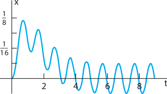
FIGURE 10.5.17.

Response `x`(`t`) to period 1 square wave input.

..................Content has been hidden....................

You can't read the all page of ebook, please click here login for view all page.

Table of Contents for 10.5 Periodic and Piecewise Continuous Input Functions

Create new playlist

Sign In

Sign Up

Table of Contents for
10.5 Periodic and Piecewise Continuous Input Functions