Search in book...
Toggle Font Controls
Create new playlist

Name your new playlist

Playlist description (optional)
Sign In

Email address

Password

Forgot Password?

or

Continue with Facebook

Continue with Google
Sign Up

Full Name

Email address

Confirm Email Address

Password

or

Continue with Facebook

Continue with Google

7.3 The Eigenvalue Method for Linear Systems

We now introduce a powerful method for constructing the general solution of a homogeneous first-order system with constant coefficients,

x' 1 x' 2 x' n = = ⋮ = a 11 x 1 a 21 x 1 a n 1 x 1 + + + a 12 x 2 a 22 x 2 a n 2 x 2 + + + \dots \dots \dots + + + a 1 n x n, a 2 n x n, a n n x n .

$\begin{array}{rcl} x_{1}^{′} & = & a_{11} x_{1} & + & a_{12} x_{2} & + & \dots & + & a_{1 n} x_{n}, \\ x_{2}^{′} & = & a_{21} x_{1} & + & a_{22} x_{2} & + & \dots & + & a_{2 n} x_{n}, \\ ⋮ \\ x_{n}^{′} & = & a_{n 1} x_{1} & + & a_{n 2} x_{2} & + & \dots & + & a_{n n} x_{n .} \end{array}$ (1)

By Theorem 3 of Section 7.2, we know that it suffices to find n linearly independent solution vectors x1, x2, …, xn $x_{1}, x_{2}, \dots, x_{n}$ ; the linear combination

x (t) = c 1 x 1 + c 2 x 2 + \dots + c n x n

$x (t) = c_{1} x_{1} + c_{2} x_{2} + \dots + c_{n} x_{n}$ (2)

with arbitrary coefficients will then be a general solution of the system in (1).

To search for the n needed linearly independent solution vectors, we proceed by analogy with the characteristic root method for solving a single homogeneous equation with constant coefficients (Section 5.3). It is reasonable to anticipate solution vectors of the form

x (t) = ⎡ ⎣ ⎢ ⎢ ⎢ ⎢ ⎢ ⎢ ⎢ x 1 x 2 x 3 ⋮ x n ⎤ ⎦ ⎥ ⎥ ⎥ ⎥ ⎥ ⎥ ⎥ = ⎡ ⎣ ⎢ ⎢ ⎢ ⎢ ⎢ ⎢ ⎢ v 1 e λ t v 2 e λ t v 3 e λ t ⋮ v n e λ t ⎤ ⎦ ⎥ ⎥ ⎥ ⎥ ⎥ ⎥ ⎥ = ⎡ ⎣ ⎢ ⎢ ⎢ ⎢ ⎢ ⎢ ⎢ v 1 v 2 v 3 ⋮ v n ⎤ ⎦ ⎥ ⎥ ⎥ ⎥ ⎥ ⎥ ⎥ e λ t = v e λ t,

$x (t) = [\begin{array}{c} x_{1} \\ x_{2} \\ x_{3} \\ ⋮ \\ x_{n} \end{array}] = [\begin{array}{c} v_{1} e^{λ t} \\ v_{2} e^{λ t} \\ v_{3} e^{λ t} \\ ⋮ \\ v_{n} e^{λ t} \end{array}] = [\begin{array}{c} v_{1} \\ v_{2} \\ v_{3} \\ ⋮ \\ v_{n} \end{array}] e^{λ t} = v e^{λ t},$ (3)

where λ, v1, v2, v3, …, vn $λ, v_{1}, v_{2}, v_{3}, \dots, v_{n}$ are appropriate scalar constants. For if we substitute

x i = v i e λ t, x' i = λ v i e λ t (i = 1, 2, \dots, n)

$x_{i} = v_{i} e^{λ t}, x_{i}^{′} = λ v_{i} e^{λ t} (i = 1, 2, \dots, n)$

in (1), then each term in the resulting equations will have the factor eλt, $e^{λ t},$ so we can cancel it throughout. This will leave us with n linear equations that—for appropriate values of λ $λ$ —we can hope to solve for values of the coefficients v1, v2, …, vn $v_{1}, v_{2}, \dots, v_{n}$ in Eq. (3), so that x(t)=veλt $x (t) = v e^{λ t}$ is, indeed, a solution of the system in (1).

To investigate this possibility, it is more efficient to write the system in (1) in the matrix form

x' = A x,

$x^{′} = A x,$ (4)

where A=[aij]. $A = [a_{i j}] .$ When we substitute the trial solution x=veλt $x = v e^{λ t}$ (having derivative x'=λveλt $x ′ = λ v e^{λ t}$ ) in Eq. (4), the result is

λ v e λ t = A v e λ t .

$λ v e^{λ t} = A v e^{λ t} .$

We cancel the nonzero scalar factor eλt $e^{λ t}$ to get

A v = λ v .

$A v = λ v .$ (5)

Recall, from Section 6.1, that Eq. (5) means that v≠0 $v \neq 0$ is an eigenvector of the matrix A associated with the eigenvalue λ. $λ .$ Our discussion of Eqs. (3)–(5) therefore provides a proof of the following theorem, which is the basis for the eigenvalue method of solving a first-order system with constant coefficients.

Recall that an eigenvalue λ $λ$ of the matrix A is a solution of the characteristic equation

| A - λ I | = det (A - λ I) = 0

$| A - λ I | = \det (A - λ I) = 0$ (6)

and that an eigenvector v associated with λ $λ$ is then a solution of the eigenvector equation

(A - λ I) v = 0 .

$(A - λ I) v = 0.$ (7)

The Eigenvalue Method

In outline, this method for solving the n×n $n \times n$ homogeneous constant-coefficient system x'=Ax $x ′ = A x$ proceeds as follows:

First, we solve the characteristic equation in (6) for the eigenvalues λ1, λ2, …, λn $λ_{1}, λ_{2}, \dots, λ_{n}$ of the matrix A.
Next, we attempt to find n linearly independent eigenvectors v1, v2, …, vn $v_{1}, v_{2}, \dots, v_{n}$ associated with these eigenvalues.
Step 2 is not always possible, but, when it is, we get n linearly independent solutions

$x 1 (t) = v 1 e λ i t, x 2 (t) = v 2 e λ 2 t, \dots, x n (t) = v n e λ n t .$ $x_{1} (t) = v_{1} e^{λ_{i} t}, x_{2} (t) = v_{2} e^{λ_{2} t}, \dots, x_{n} (t) = v_{n} e^{λ n t} .$ (8)

In this case the general solution of x'=Ax $x ′ = A x$ is a linear combination

$x (t) = c 1 x 1 (t) + c 2 x 2 (t) + \dots + c n x n (t)$ $x (t) = c_{1} x_{1} (t) + c_{2} x_{2} (t) + \dots + c_{n} x_{n} (t)$

of these n solutions.

We will discuss separately the various cases that can occur, depending on whether the eigenvalues are distinct or repeated, real or complex. The case of repeated eigenvalues—multiple roots of the characteristic equation—will be deferred to Section 7.6.

Distinct Real Eigenvalues

If the eigenvalues λ1, λ2, …, λn $λ_{1}, λ_{2}, \dots, λ_{n}$ are real and distinct, then we substitute each of them in turn in Eq. (7) and solve for the associated eigenvectors v1, v2, …, vn. $v_{1}, v_{2}, \dots, v_{n} .$ It then follows from Theorem 2 in Section 6.2 that the particular solutions given in (8) are linearly independent. (In any particular example, such linear independence can always be verified by using the Wronskian determinant of Section 7.2.) The following example illustrates the eigenvalue method.

Example 1

Find a general solution of the system

x' 1 x' 2 = = 4 x 1 3 x 1 + - 2 x 2, x 2 .

$\begin{array}{rcrcr} x_{1}^{′} & = & 4 x_{1} & + & 2 x_{2}, \\ x_{2}^{′} & = & 3 x_{1} & - & x_{2} . \end{array}$ (9)

Solution

The matrix form of the system in (9) is

x' = [43 2 - 1] x .

$x^{′} = [\begin{array}{r} 4 & 2 \\ 3 & - 1 \end{array}] x .$ (10)

The characteristic equation of the coefficient matrix is

∣ ∣ ∣ 4 - λ 3 2 - 1 - λ ∣ ∣ ∣ = = (4 - λ) (- 1 - λ) - 6 λ 2 - 3 λ - 10 = (λ + 2) (λ - 5) = 0,

$\begin{array}{rcl} | \begin{array}{c} 4 - λ & 2 \\ 3 & - 1 - λ \end{array} | & = & (4 - λ) (- 1 - λ) - 6 \\ = & λ^{2} - 3 λ - 10 = (λ + 2) (λ - 5) = 0, \end{array}$

so we have the distinct real eigenvalues λ1=−2 $λ_{1} = - 2$ and λ2=5 $λ_{2} = 5$ .

For the coefficient matrix A in Eq. (10), the eigenvector equation (A−λI)v=0 $(A - λ I) v = 0$ takes the form

[4 - λ 3 2 - 1 - λ] [a b] = [00]

$[\begin{array}{c} 4 - λ & 2 \\ 3 & - 1 - λ \end{array}] [\begin{array}{c} a \\ b \end{array}] = [\begin{array}{c} 0 \\ 0 \end{array}]$ (11)

for the associated eigenvector v=[ab]T. $v = {[\begin{array}{l} a & b \end{array}]}^{T} .$

Case 1: λ1=−2. $λ_{1} = - 2 .$ Substitution of the first eigenvalue λ1=−2 $λ_{1} = - 2$ in Eq. (11) yields the system

$[\begin{array}{r} 6 & 2 \\ 3 & 1 \end{array}] [\begin{array}{c} a \\ b \end{array}] = [\begin{array}{c} 0 \\ 0 \end{array}]$

—that is, the two scalar equations

$\begin{array}{rcrcl} 6 a & + & 2 b & = & 0, \\ 3 a & + & b & = & 0. \end{array}$ (12)

In contrast with the typical nonsingular (algebraic) linear system that has a unique solution, the homogeneous linear system in (12) is singular—the two scalar equations obviously are equivalent (each being a multiple of the other). Therefore, Eq. (12) has infinitely many nonzero solutions—we can choose a arbitrarily (but nonzero) and then solve for b.

Substitution of an eigenvalue $λ$ in the eigenvector equation $(A - λ I) v = 0$ always yields a singular homogeneous linear system, and among its infinity of solutions we generally seek a “simple” solution with small integer values (if possible). Looking at the second equation in (12), the choice $a = 1$ yields $b = - 3,$ and thus

$v_{1} = [\begin{array}{r} 1 \\ - 3 \end{array}]$

is an eigenvector associated with $λ_{1} = - 2$ (as is any nonzero constant multiple of $v_{1}$ ).

Remark

If, instead of the “simplest” choice $a = 1, b = - 3,$ we had made another choice $a = c, b = - 3 c,$ we would have obtained the eigenvector

$v_{1} = [\begin{array}{r} c \\ - 3 c \end{array}] = c [\begin{array}{r} 1 \\ - 3 \end{array}] .$

Because this is a constant multiple of our previous result, any choice we make leads to (a constant multiple of ) the same solution

$x_{1} (t) = [\begin{array}{r} 1 \\ - 3 \end{array}] e^{- 2 t} .$

Case 2: $λ_{2} = 5 .$ Substitution of the second eigenvalue $λ = 5$ in (11) yields the pair

$\begin{array}{rcl} - a + 2 b & = & 0, \\ 3 a - 6 b & = & 0 \end{array}$ (13)

of equivalent scalar equations. With $b = 1$ in the first equation we get $a = 2,$ so

$v_{2} = [\begin{array}{l} 2 \\ 1 \end{array}]$

is an eigenvector associated with $λ_{2} = 5 .$ A different choice— $a = 2 c, b = c$ —would merely give a [constant] multiple of $v_{2}$ .

These two eigenvalues and their associated eigenvectors yield the two solutions

$x_{1} (t) = [\begin{array}{r} 1 \\ - 3 \end{array}] e^{- 2 t} and x_{2} (t) = [\begin{array}{l} 2 \\ 1 \end{array}] e^{5 t} .$

They are linearly independent, because their Wronskian

$| \begin{array}{c} e^{- 2 t} & 2 e^{5 t} \\ - 3 e^{- 2 t} & e^{5 t} \end{array} | = 7 e^{3 t}$

is nonzero. Hence a general solution of the system in (10) is

$x (t) = c_{1} x_{1} (t) + c_{2} x_{2} (t) = c_{1} [\begin{array}{r} 1 \\ - 3 \end{array}] e^{- 2 t} + c_{2} [\begin{array}{r} 2 \\ 1 \end{array}] e^{5 t};$

in scalar form,

$\begin{array}{rcrcr} x_{1} (t) & = & c_{1} e^{- 2 t} & + & 2 c_{2} e^{5 t}, \\ x_{2} (t) & = & - 3 c_{1} e^{- 2 t} & + & c_{2} e^{5 t} . \end{array}$

Figure 7.3.1 shows some typical solution curves of the system in (10). We see two families of hyperbolas sharing the same pair of asymptotes: the line $x_{1} = 2 x_{2}$ obtained from the general solution with $c_{1} = 0,$ and the line $x_{2} = - 3 x_{1}$ obtained with $c_{2} = 0 .$ Given initial values $x_{1} (0) = b_{1}, x_{2} (0) = b_{2},$ it is apparent from the figure that

If $(b_{1}, b_{2})$ lies to the right of the line $x_{2} = - 3 x_{1},$ then $x_{1} (t)$ and $x_{2} (t)$ both tend to $+ \infty$ as $t \to + \infty$ ;
If $(b_{1}, b_{2})$ lies to the left of the line $x_{2} = - 3 x_{1},$ then $x_{1} (t)$ and $x_{2} (t)$ both tend to $- \infty$ as $t \to + \infty$ .

FIGURE 7.3.1.

Direction field and solution curves for the linear system $x_{1}^{′} = 4 x_{1} + 2 x_{2}, x_{2}^{′} = 3 x_{1} - x_{2}$ of Example 1.

Remark

As in Example 1, it is convenient when discussing a linear system $x ′ = A x$ to use vectors $x_{1}, x_{2}, \dots, x_{n}$ to denote different vector-valued solutions of the system, whereas the scalars $x_{1}, x_{2}, \dots, x_{n}$ denote the components of a single vector-valued solution x.

Compartmental Analysis

Frequently, a complex process or system can be broken down into simpler subsystems or “compartments” that can be analyzed separately. The whole system can then be modeled by describing the interactions between the various compartments. Thus a chemical plant may consist of a succession of separate stages (or even physical compartments) in which various reactants and products combine or are mixed. It may happen that a single differential equation describes each compartment of the system; then the whole physical system is modeled by a system of differential equations.

As a simple example of a three-stage system, Fig. 7.3.2 shows three brine tanks containing $V_{1}, V_{2},$ and $V_{3}$ gallons of brine, respectively. Fresh water flows into tank 1, while mixed brine flows from tank 1 into tank 2, from tank 2 into tank 3, and out of tank 3. Let $x_{i} (t)$ denote the amount (in pounds) of salt in tank i at time t, for $i = 1, 2,$ and 3. If each flow rate is r gallons per minute, then a simple accounting of salt concentrations, as in Example 2 of Section 7.1, yields the first-order system

$\begin{array}{rcl} x_{1}^{′} & = & - k_{1} x_{1}, \\ x_{2}^{′} & = & k_{1} x_{1} - k_{2} x_{2}, \\ x_{3}^{′} & = & k_{2} x_{2} - k_{3} x_{3}, \end{array}$ (14)

where

$\begin{array}{l} k_{i} = \frac{r}{V_{i}}, & i = 1, 2, 3. \end{array}$ (15)

Example 2

Three brine tanks If $V_{1} = 20, V_{2} = 40, V_{3} = 50, r = 10$ (gal/min), and the initial amounts of salt in the three brine tanks, in pounds, are

$x_{1} (0) = 15, x_{2} (0) = x_{3} (0) = 0,$

find the amount of salt in each tank at time $t ≧ 0$ .

Solution

Substituting the given numerical values in (14) and (15), we get the initial value problem

$\begin{array}{l} x^{′} (t) = [\begin{array}{r} - 0.5 & 0.0 & 0.0 \\ 0.5 & - 0.25 & 0.0 \\ 0.0 & 0.25 & - 0.2 \end{array}] x, & x (0) = [\begin{array}{r} 15 \\ 0 \\ 0 \end{array}] \end{array}$ (16)

for the vector $x (t) = {[\begin{array}{l} x_{1} (t) & x_{2} (t) & x_{3} (t) \end{array}]}^{T} .$ The simple form of the matrix

$A - λ I = [\begin{array}{c} - 0.5 - λ & 0.0 & 0.0 \\ 0.5 & - 0.25 - λ & 0.0 \\ 0.0 & 0.25 & - 0.2 - λ \end{array}]$ (17)

leads readily to the characteristic equation

$| A - λ I | = (- 0.5 - λ) (- 0.25 - λ) (- 0.2 - λ) = 0.$

Thus, the coefficient matrix A in (16) has the distinct eigenvalues $λ_{1} = - 0.5, λ_{2} = - 0.25,$ and $λ_{3} = - 0.2$ and therefore has three linearly independent eigenvectors.

FIGURE 7.3.2.

The three brine tanks of Example 2.

Case 1: $λ_{1} = - 0.5 .$ Substituting $λ = - 0.5$ in (17), we get the equation

$[A + (0.5) \cdot I] v = [\begin{array}{c} 0.0 & 0.0 & 0.0 \\ 0.5 & 0.25 & 0.0 \\ 0.0 & 0.25 & 0.3 \end{array}] [\begin{array}{c} a \\ b \\ c \end{array}] = [\begin{array}{c} 0 \\ 0 \\ 0 \end{array}]$

for the associated eigenvector $v = {[\begin{array}{l} a & b & c \end{array}]}^{T} .$ The last two rows, after division by 0.25 and 0.05, respectively, yield the scalar equations

$\begin{array}{rcrcl} 2 a & + & b & = & 0, \\ 5 b & + & 6 c & = & 0. \end{array}$

The second equation is satisfied by $b = - 6$ and $c = 5,$ and then the first equation gives $a = 3 .$ Thus the eigenvector

$v_{1} = {[\begin{array}{l} 3 & - 6 & 5 \end{array}]}^{T}$

is associated with the eigenvalue $λ_{1} = - 0.5$ .

Case 2: $λ_{2} = - 0.25 .$ Substituting $λ = - 0.25$ in (17), we get the equation

$[A + (0.25) \cdot I] v = [\begin{array}{c} - 0.25 & 0 & 0 \\ 0.5 & 0 & 0 \\ 0 & 0.25 & 0.05 \end{array}] [\begin{array}{c} a \\ b \\ c \end{array}] = [\begin{array}{c} 0 \\ 0 \\ 0 \end{array}]$

for the associated eigenvector $v = {[\begin{array}{l} a & b & c \end{array}]}^{T} .$ Each of the first two rows implies that $a = 0,$ and division of the third row by 0.05 gives the equation

$5 b + c = 0,$

which is satisfied by $b = 1, c = - 5 .$ Thus the eigenvector

$v_{2} = {[\begin{array}{l} 0 & 1 & - 5 \end{array}]}^{T}$

is associated with the eigenvalue $λ_{2} = - 0.25$ .

Case 3: $λ_{3} = - 0.2 .$ Substituting $λ = - 0.2$ in (17), we get the equation

$[A + (0.2) \cdot I] v = [\begin{array}{r} - 0.3 & 0.0 & 0.0 \\ 0.5 & - 0.05 & 0.0 \\ 0.0 & 0.25 & 0.0 \end{array}] [\begin{array}{c} a \\ b \\ c \end{array}] = [\begin{array}{c} 0 \\ 0 \\ 0 \end{array}]$

for the eigenvector v. The first and third rows imply that $a = 0,$ and $b = 0,$ respectively, but the all-zero third column leaves c arbitrary (but nonzero). Thus

$v_{3} = {[\begin{array}{l} 0 & 0 & 1 \end{array}]}^{T}$

is an eigenvector associated with $λ_{3} = - 0.2$ .

The general solution

$x (t) = c_{1} v_{1} e^{λ_{1} t} + c_{2} v_{2} e^{λ_{2} t} + c_{3} v_{3} e^{λ_{3} t}$

therefore takes the form

$x (t) = c_{1} [\begin{array}{r} 3 \\ - 6 \\ 3 \end{array}] e^{(- 0.5) t} + c_{2} [\begin{array}{r} 0 \\ 1 \\ - 5 \end{array}] e^{(- 0.25) t} + c_{3} [\begin{array}{c} 0 \\ 0 \\ 1 \end{array}] e^{(- 0.2) t} .$

The resulting scalar equations are

$\begin{array}{rclllll} x_{1} (t) & = & 3 c_{1} e^{(- 0.5) t}, \\ x_{2} (t) & = & - 6 c_{1} e^{(- 0.5) t} & + & c_{2} e^{(- 0.25) t}, \\ x_{3} (t) & = & 5 c_{1} e^{(- 0.5) t} & - & 5 c_{2} e^{(- 0.25) t} & + & c_{3} e^{(- 0.2) t} . \end{array}$

When we impose the initial conditions $x_{1} (0) = 15, x_{2} (0) = x_{3} (0) = 0,$ we get the equations

$\begin{array}{rcrcl} 3 c_{1} & = & 15, \\ - 6 c_{1} & + & c_{2} & = & 0, \\ 5 c_{1} & - & 5 c_{2} & + & c_{3} & = & 0 \end{array}$

that are readily solved (in turn) for $c_{1} = 5, c_{2} = 30,$ and $c_{3} = 125 .$ Thus, finally, the amounts of salt at time t in the three brine tanks are given by

$\begin{array}{rcl} x_{1} (t) & = & 15 e^{(- 0.5) t}, \\ x_{2} (t) & = & - 30 e^{(- 0.5) t} + 30 e^{(- 0.25) t}, \\ x_{3} (t) & = & 25 e^{(- 0.5) t} - 150 e^{(- 0.25) t} + 125 e^{(- 0.2) t} . \end{array}$

Figure 7.3.3 shows the graphs of $x_{1} (t), x_{2} (t),$ and $x_{3} (t) .$ As we would expect, tank 1 is rapidly “flushed” by the incoming fresh water, and $x_{1} (t) \to 0$ as $t \to + \infty .$ The amounts $x_{2} (t)$ and $x_{3} (t)$ of salt in tanks 2 and 3 peak in turn and then approach zero as the whole three-tank system is purged of salt as $t \to + \infty$ .

FIGURE 7.3.3.

The salt content functions of Example 2.

Complex Eigenvalues

Even if some of the eigenvalues are complex, so long as they are distinct the method described previously still yields n linearly independent solutions. The only complication is that the eigenvectors associated with complex eigenvalues are ordinarily complex-valued, so we will have complex-valued solutions.

To obtain real-valued solutions, we note that—because we are assuming that the matrix A has only real entries—the coefficients in the characteristic equation will all be real. Consequently any complex eigenvalues must appear in complex-conjugate pairs. Suppose, then, that $λ = p + q i$ and $\overset{̲}{λ} = p - q i$ are such a pair of eigenvalues. If v is an eigenvector associated with $λ,$ so that

$(A - λ I) v = 0,$

then taking complex conjugates in this equation yields

$(A - \bar{λ} I) \bar{v} = 0$

since $\overset{̲}{A} = A$ and $\overset{̲}{I} = I$ (these matrices being real) and the conjugate of a complex product is the product of the conjugates of the factors. Thus the conjugate $\overset{̲}{v}$ of v is an eigenvector associated with $\overset{̲}{λ} .$ Of course, the conjugate of a vector is defined componentwise; if

$v = [\begin{array}{c} a_{1} + b_{1} i \\ a 2 + b_{2} i \\ ⋮ \\ a_{n} + b_{n} i \end{array}] = [\begin{array}{c} a_{1} \\ a_{2} \\ ⋮ \\ a_{n} \end{array}] + [\begin{array}{c} b_{1} \\ b_{2} \\ ⋮ \\ b_{n} \end{array}] i = a + b i,$ (18)

then $\overset{̲}{v} = a - b i .$ The complex-valued solution associated with $λ$ and v is then

$x (t) = v e^{λ t} = v e^{(p + q i) t} = (a + b i) e^{p t} (\cos q t + i \sin q t)$

—that is,

$x (t) = e^{p t} (a \cos q t - b \sin q t) + i e^{p t} (b \cos q t + a \sin q t) .$ (19)

Because the real and imaginary parts of a complex-valued solution are also solutions, we thus get the two real-valued solutions

$\begin{array}{rcl} x_{1} (t) & = & Re [x (t)] = e^{p t} (a \cos q t - b \sin q t), \\ x_{2} (t) & = & Im [x (t)] = e^{p t} (b \cos q t + a \sin q t) \end{array}$ (20)

associated with the complex conjugate eigenvalues $p \pm q i .$ It is easy to check that the same two real-valued solutions result from taking real and imaginary parts of $\overset{̲}{v} e^{\overset{̲}{λ} t} .$ Rather than memorizing the formulas in (20), it is preferable in a specific example to proceed as follows:

First, find explicitly a single complex-valued solution x(t) associated with the complex eigenvalue $λ$ ;
Then, find the real and imaginary parts $x_{1} (t)$ and $x_{2} (t),$ to get two independent real-valued solutions corresponding to the two complex conjugate eigenvalues $λ$ and $\overset{̲}{λ}$ .

Example 3

Find a general solution of the system

$\begin{array}{rcl} \frac{d x_{1}}{d t} & = & 4 x_{1} - 3 x_{2}, \\ \frac{d x_{2}}{d t} & = & 3 x_{1} + 4 x_{2} . \end{array}$ (21)

Solution

The coefficient matrix

$A = [\begin{array}{r} 4 & - 3 \\ 3 & 4 \end{array}]$

has the characteristic equation

$| A - λ I | = | \begin{array}{c} 4 - λ & - 3 \\ 3 & 4 - λ \end{array} | = {(4 - λ)}^{2} + 9 = 0$

and hence has the complex conjugate eigenvalues $λ = 4 - 3 i$ and $\overset{̲}{λ} = 4 + 3 i$ .

Substituting $λ = 4 - 3 i$ in the eigenvector equation $(A - λ I) v = 0,$ we get the equation

$[A - (4 - 3 i) \cdot I] v = [\begin{array}{r} 3 i & - 3 \\ 3 & 3 i \end{array}] [\begin{array}{c} a \\ b \end{array}] = [\begin{array}{c} 0 \\ 0 \end{array}]$

for an associated eigenvalue $v = {[\begin{array}{l} a & b \end{array}]}^{T} .$ Division of each row by 3 yields the two scalar equations

$\begin{array}{rcrcl} i a & - & b & = & 0, \\ a & + & i b & = & 0, \end{array}$

each of which is satisfied by $a = 1$ and $b = i .$ Thus, $v = {[\begin{array}{l} 1 & i \end{array}]}^{T}$ is a complex eigenvector associated with the complex eigenvalue $λ = 4 - 3 i$ .

The corresponding complex-valued solution $x (t) = v e^{λ t}$ of $x ′ = A x$ is then

$x (t) = [\begin{array}{c} 1 \\ i \end{array}] e^{(4 - 3 i) t} = [\begin{array}{c} 1 \\ i \end{array}] e^{4 t} (\cos 3 t - i \sin 3 t) = e^{4 t} [\begin{array}{rcr} \cos 3 t & - & i \sin 3 t \\ i \cos 3 t & + & \sin 3 t \end{array}] .$

The real and imaginary parts of x(t) are the real-valued solutions

$x_{1} (t) = e^{4 t} [\begin{array}{c} \cos 3 t \\ \sin 3 t \end{array}] and x_{2} (t) = e^{4 t} [\begin{array}{c} - \sin 3 t \\ \cos 3 t \end{array}] .$

A real-valued general solution of $x ′ = A x$ is then given by

$x (t) = c_{1} x_{1} (t) + c_{2} x_{2} (t) = e^{4 t} [\begin{array}{c} c_{1} \cos 3 t - c_{2} \sin 3 t \\ c_{1} \sin 3 t + c_{2} \cos 3 t \end{array}] .$

Finally, a general solution of the system in (21) in scalar form is

$\begin{array}{rcl} x_{1} (t) & = & e^{4 t} (c_{1} \cos 3 t - c_{2} \sin 3 t), \\ x_{2} (t) & = & e^{4 t} (c_{1} \sin 3 t + c_{2} \cos 3 t) . \end{array}$

Figure 7.3.4 shows some typical solution curves of the system in (21). Each appears to spiral counterclockwise as it emanates from the origin in the $x_{1} x_{2}$ -plane. Actually, because of the factor $e^{4 t}$ in the general solution, we see that

Along each solution curve, the point $(x_{1} (t), x_{2} (t))$ approaches the origin as $t \to - \infty,$ whereas
The absolute values of $x_{1} (t)$ and $x_{2} (t)$ both increase without bound as $t \to + \infty$ .

FIGURE 7.3.4.

Direction field and solution curves for the linear system $x_{1} ′ = 4 x_{1} - 3 x_{2}, x_{2} ′ = 3 x_{1} + 4 x_{2}$ of Example 3.

Figure 7.3.5 shows a “closed” system of three brine tanks with volumes $V_{1}, V_{2},$ and $V_{3} .$ The difference between this system and the “open” system of Fig. 7.3.2 is that now the inflow to tank 1 is the outflow from tank 3. With the same notation as in Example 2, the appropriate modification of Eq. (14) is

$\begin{array}{rcrclcl} \frac{d x_{1}}{d t} & = & - k_{1} x_{1} & + k_{3} x_{3}, \\ \frac{d x_{2}}{d t} & = & k_{1} x_{1} & - k_{2} x_{2}, \\ \frac{d x_{3}}{d t} & = & k_{2} x_{2} & - k_{3} x_{3}, \end{array}$ (22)

where $k_{i} = r / V_{i}$ as in (15).

Example 4

Find the amounts $x_{1} (t), x_{2} (t),$ and $x_{3} (t)$ of salt at time t in the three brine tanks of Fig. 7.3.5 if $V_{1} = 50$ gal, $V_{2} = 25$ gal, $V_{3} = 50$ gal, and $r = 10$ gal/min.

Solution

With the given numerical values, (22) takes the form

$\frac{d x}{d t} = [\begin{array}{r} - 0.2 & 0 & 0.2 \\ 0.2 & - 0.4 & 0 \\ 0 & 0.4 & - 0.2 \end{array}] x,$ (23)

where $x = {[\begin{array}{r} x_{1} & x_{2} & x_{3} \end{array}]}^{T}$ as usual. When we expand the determinant of the matrix

$A - λ \cdot I = [\begin{array}{c} - 0.2 - λ & 0.0 & 0.2 \\ 0.2 & - 0.4 - λ & 0.0 \\ 0.0 & 0.4 & - 0.2 - λ \end{array}]$ (24)

along its first row, we find that the characteristic equation of A is

$\begin{array}{l} (- 0.2 - λ) (- 0.4 - λ) (- 0.2 - λ) + (0.2) (0.2) (0.4) \\ \begin{array}{l} = - λ^{3} - (0.8) \cdot λ^{2} - (0.2) \cdot λ \\ = - λ [{(λ + 0.4)}^{2} + {(0.2)}^{2}] = 0. \end{array} \end{array}$

Thus A has the zero eigenvalue $λ_{0} = 0$ and the complex conjugate eigenvalues $λ,$ $\overset{̲}{λ} = - 0.4 \pm (0.2) i .$ We anticipate one solution corresponding to the zero eigenvalue and two additional linearly independent solutions corresponding to the complex conjugate eigenvalues.

Case 1: $λ_{0} = 0 .$ Substitution of $λ = 0$ in Eq. (24) gives the eigenvector equation

$(A - 0 \cdot I) v = [\begin{array}{r} - 0.2 & 0.0 & 0.2 \\ 0.2 & - 0.4 & 0.0 \\ 0.0 & 0.4 & - 0.2 \end{array}] [\begin{array}{c} a \\ b \\ c \end{array}] = [\begin{array}{c} 0 \\ 0 \\ 0 \end{array}]$ (25)

for $v = {[\begin{array}{l} a & b & c \end{array}]}^{T} .$ The first row gives $a = c$ and the second row gives $a = 2 b,$ so $v_{0} = {[\begin{array}{l} 2 & 1 & 2 \end{array}]}^{T}$ is an eigenvector associated with the eigenvalue $λ_{0} = 0 .$ The corresponding solution $x_{0} (t) = v_{0} e^{λ_{0} t}$ of Eq. (23) is the constant solution

$x_{0} (t) = [\begin{array}{c} 2 \\ 1 \\ 2 \end{array}] .$ (26)

Case 2: $λ = - 0.4 - (0.2) i .$ Substitution of $λ = - 0.4 - (0.2) i$ in Eq. (24) gives the eigenvector equation

$[A - (- 0.4 - (0.2) i) I] v = [\begin{array}{c} 0.2 + (0.2) i & 0.0 & 0.2 \\ 0.2 & (0.2) i & 0.0 \\ 0.0 & 0.4 & 0.2 + (0.2) i \end{array}] [\begin{array}{c} a \\ b \\ c \end{array}] = [\begin{array}{c} 0 \\ 0 \\ 0 \end{array}] .$

The second equation $(0.2) a + (0.2) i b = 0$ is satisfied by $a = 1$ and $b = i .$ Then the first equation

$[0.2 + (0.2) i] a + (0.2) c = 0$

gives $c = - 1 - i .$ Thus, $v = {[\begin{array}{r} 1 & i & (- 1 - i) \end{array}]}^{T}$ is a complex eigenvector associated with the complex eigenvalue $λ = - 0.4 - (0.2) i$ .

The corresponding complex-valued solution $x (t) = v e^{λ t}$ of (23) is

$\begin{array}{rcl} x (t) & = & {[\begin{array}{r} 1 & i & - 1 & - i \end{array}]}^{T} e^{(- 0.4 - 0.2 i) t} \\ = & {[\begin{array}{r} 1 & i & - 1 & - i \end{array}]}^{T} e^{(- 0.4) t} (\cos 0.2 t - i \sin 0.2 t) \\ = & e^{(- 0.4) t} [\begin{array}{c} \cos 0.2 t - i \sin 0.2 t \\ \sin 0.2 t + i \cos 0.2 t \\ - \cos 0.2 t - \sin 0.2 t - i \cos 0.2 t + i \sin 0.2 t \end{array}] . \end{array}$

The real and imaginary parts of x(t) are the real-valued solutions

$\begin{array}{rcl} x_{1} (t) & = & e^{(- 0.4) t} [\begin{array}{c} \cos 0.2 t \\ \sin 0.2 t \\ - \cos 0.2 t - \sin 0.2 t \end{array}], \\ x_{2} (t) & = & e^{(- 0.4) t} [\begin{array}{c} - \sin 0.2 t \\ \cos 0.2 t \\ - \cos 0.2 t + \sin 0.2 t \end{array}] . \end{array}$ (27)

The general solution

$x (t) = c_{0} x_{0} (t) + c_{1} x_{1} (t) + c_{2} x_{2} (t)$

has scalar components

$\begin{array}{rcrcl} x_{1} (t) & = & 2 c_{0} & + & e^{(- 0.4) t} (c_{1} \cos 0.2 t - c_{2} \sin 0.2 t), \\ x_{2} (t) & = & c_{0} & + & e^{(- 0.4) t} (c_{1} \sin 0.2 t + c_{2} \cos 0.2 t), \\ x_{3} (t) & = & 2 c_{0} & + & e^{(- 0.4) t} [(- c_{1} - c_{2}) \cos 0.2 t + (- c_{1} + c_{2}) \sin 0.2 t] \end{array}$ (28)

giving the amounts of salt in the three tanks at time t.

Observe that

$x_{1} (t) + x_{2} (t) + x_{3} (t) \equiv 5 c_{0} .$ (29)

Of course, the total amount of salt in the closed system is constant; the constant $c_{0}$ in (29) is one-fifth the total amount of salt. Because of the factors of $e^{(- 0.4) t}$ in (28), we see that

$\begin{array}{l} \lim_{t \to \infty} x_{1} (t) = 2 c_{0}, & \lim_{t \to \infty} x_{2} (t) = c_{0}, & and & \lim_{t \to \infty} x_{3} (t) = 2 c_{0} . \end{array}$

Thus, as $t \to + \infty$ the salt in the system approaches a steady-state distribution with 40% of the salt in each of the two 50-gallon tanks and 20% in the 25-gallon tank. So whatever the initial distribution of salt among the three tanks, the limiting distribution is one of uniform concentration throughout the system. Figure 7.3.6 shows the graphs of the three solution functions with $c_{0} = 10, c_{1} = 30,$ and $c_{2} = - 10,$ in which case

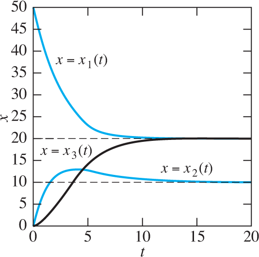
$\begin{array}{l} x_{1} (0) = 50 & and & x_{2} (0) = x_{3} (0) = 0. \end{array}$

FIGURE 7.3.6.

The salt content functions of Example 4.

7.3 Problems

In Problems 1 through 16, apply the eigenvalue method of this section to find a general solution of the given system. If initial values are given, find also the corresponding particular solution. For each problem, use a computer system or graphing calculator to construct a direction field and typical solution curves for the given system.

$x_{1}^{′} = x_{1} + 2 x_{2}, x_{2}^{′} = 2 x_{1} + x_{2}$
$x_{1}^{′} = 2 x_{1} + 3 x_{2}, x_{2}^{′} = 2 x_{1} + x_{2}$
$x_{1}^{′} = 3 x_{1} + 4 x_{2}, x_{2}^{′} = 3 x_{1} + 2 x_{2}; x_{1} (0) = x_{2} (0) = 1$
$x_{1}^{′} = 4 x_{1} + x_{2}, x_{2}^{′} = 6 x_{1} - x_{2}$
$x_{1}^{′} = 6 x_{1} - 7 x_{2}, x_{2}^{′} = x_{1} - 2 x_{2}$
$x_{1}^{′} = 9 x_{1} + 5 x_{2}, x_{2}^{′} = - 6 x_{1} - 2 x_{2}; x_{1} (0) = 1, x_{2} (0) = 0$
$x_{1}^{′} = - 3 x_{1} + 4 x_{2}, x_{2}^{′} = 6 x_{1} - 5 x_{2}$
$x_{1}^{′} = x_{1} - 5 x_{2}, x_{2}^{′} = x_{1} - x_{2}$
$x_{1}^{′} = 2 x_{1} - 5 x_{2}, x_{2}^{′} = 4 x_{1} - 2 x_{2}; x_{1} (0) = 2, x_{2} (0) = 3$
$x_{1}^{′} = - 3 x_{1} - 2 x_{2}, x_{2}^{′} = 9 x_{1} - 3 x_{2}$
$x_{1}^{′} = x_{1} - 2 x_{2}, x_{2}^{′} = 2 x_{1} + x_{2}; x_{1} (0) = 0, x_{2} (0) = 4$
$x_{1}^{′} = x_{1} - 5 x_{2}, x_{2}^{′} = x_{1} + 3 x_{2}$
$x_{1}^{′} = 5 x_{1} - 9 x_{2}, x_{2}^{′} = 2 x_{1} - x_{2}$
$x_{1}^{′} = 3 x_{1} - 4 x_{2}, x_{2}^{′} = 4 x_{1} + 3 x_{2}$
$x_{1}^{′} = 7 x_{1} - 5 x_{2}, x_{2}^{′} = 4 x_{1} + 3 x_{2}$
$x_{1}^{′} = - 50 x_{1} + 20 x_{2}, x_{2}^{′} = 100 x_{1} - 60 x_{2}$

In Problems 17 through 25, the eigenvalues of the coefficient matrix can be found by inspection and factoring. Apply the eigenvalue method to find a general solution of each system.

$x_{1}^{′} = 4 x_{1} + x_{2} + 4 x_{3}, x_{2}^{′} = x_{1} + 7 x_{2} + x_{3}, x_{3}^{′} = 4 x_{1} + x_{2} + 4 x_{3}$
$x_{1}^{′} = x_{1} + 2 x_{2} + 2 x_{3}, x_{2}^{′} = 2 x_{1} + 7 x_{2} + x_{3}, x_{3}^{′} = 2 x_{1} + x_{2} + 7 x_{3}$
$x_{1}^{′} = 4 x_{1} + x_{2} + x_{3}, x_{2}^{′} = x_{1} + 4 x_{2} + x_{3}, x_{3}^{′} = x_{1} + x_{2} + 4 x_{3}$
$x_{1}^{′} = 5 x_{1} + x_{2} + 3 x_{3}, x_{2}^{′} = x_{1} + 7 x_{2} + x_{3}, x_{3}^{′} = 3 x_{1} + x_{2} + 5 x_{3}$
$x_{1}^{′} = 5 x_{1} - 6 x_{3}, x_{2}^{′} = 2 x_{1} - x_{2} - 2 x_{3}, x_{3}^{′} = 4 x_{1} - 2 x_{2} - 4 x_{3}$
$x_{1}^{′} = 3 x_{1} + 2 x_{2} + 2 x_{3}, x_{2}^{′} = - 5 x_{1} - 4 x_{2} - 2 x_{3}, x_{3}^{′} = 5 x_{1} + 5 x_{2} + 3 x_{3}$
$x_{1}^{′} = 3 x_{1} + x_{2} + x_{3}, x_{2}^{′} = - 5 x_{1} - 3 x_{2} - x_{3}, x_{3}^{′} = 5 x_{1} + 5 x_{2} + 3 x_{3}$
$x_{1}^{′} = 2 x_{1} + x_{2} - x_{3}, x_{2}^{′} = - 4 x_{1} - 3 x_{2} - x_{3}, x_{3}^{′} = 4 x_{1} + 4 x_{2} + 2 x_{3}$
$x_{1}^{′} = 5 x_{1} + 5 x_{2} + 2 x_{3}, x_{2}^{′} = - 6 x_{1} - 6 x_{2} - 5 x_{3}, x_{3}^{′} = 6 x_{1} + 6 x_{2} + 5 x_{3}$
Find the particular solution of the system

$\begin{array}{rcrcrcl} \frac{d x_{1}}{d t} & = & 3 x_{1} & + & x_{3}, \\ \frac{d x_{2}}{d t} & = & 9 x_{1} & - & x_{2} & + & 2 x_{3}, \\ \frac{d x_{3}}{d t} & = & - 9 x_{1} & + & 4 x_{2} & - & x_{3} \end{array}$

that satisfies the initial conditions $x_{1} (0) = 0, x_{2} (0) = 0, x_{3} (0) = 17$ .

Cascading Brine Tanks

The amounts $x_{1} (t)$ and $x_{2} (t)$ of salt in the two brine tanks of Fig. 7.3.7 satisfy the differential equations

$\begin{array}{l} \frac{d x_{1}}{d t} = - k_{1} x_{1}, & \frac{d x_{2}}{d t} = k_{1} x_{1} - k_{2} x_{2}, \end{array}$

where $k_{i} = r / V_{i}$ for $i = 1, 2 .$ In Problems 27 and 28 the volumes $V_{1}$ and $V_{2}$ are given. First solve for $x_{1} (t)$ and $x_{2} (t),$ assuming that $r = 10$ (gal/min), $x_{1} (0) = 15$ (lb), and $x_{2} (0) = 0 .$ Then find the maximum amount of salt ever in tank 2. Finally, construct a figure showing the graphs of $x_{1} (t)$ and $x_{2} (t)$ .

FIGURE 7.3.7.

The two brine tanks of Problems 27 and 28.

$V_{1} = 50$ (gal), $V_{2} = 25$ (gal)
$V_{1} = 25$ (gal), $V_{2} = 40$ (gal)

Interconnected Brine Tanks

The amounts $x_{1} (t)$ and $x_{2} (t)$ of salt in the two brine tanks of Fig. 7.3.8 satisfy the differential equations

$\begin{array}{l} \frac{d x_{1}}{d t} = - k_{1} x_{1} + k_{2} x_{2}, & \frac{d x_{2}}{d t} = k_{1} x_{1} - k_{2} x_{2}, \end{array}$

where $k_{i} = r / V_{i}$ as usual. In Problems 29 and 30, solve for $x_{1} (t)$ and $x_{2} (t),$ assuming that $r = 10$ (gal/min), $x_{1} (0) = 15$ (lb), and $x_{2} (0) = 0 .$ Then construct a figure showing the graphs of $x_{1} (t)$ and $x_{2} (t)$ .

FIGURE 7.3.8.

The two brine tanks of Problems 29 and 30.

$V_{1} = 50$ (gal), $V_{2} = 25$ (gal)
$V_{1} = 25$ (gal), $V_{2} = 40$ (gal)

Open Three-Tank System

Problems 31 through 34 deal with the open three-tank system of Fig. 7.3.2. Fresh water flows into tank 1; mixed brine flows from tank 1 into tank 2, from tank 2 into tank 3, and out of tank 3; all at the given flow rate r gallons per minute. The initial amounts $x_{1} (0) = x_{0}$ (lb), $x_{2} (0) = 0,$ and $x_{3} (0) = 0$ of salt in the three tanks are given, as are their volumes $V_{1}, V_{2},$ and $V_{3}$ (in gallons). First solve for the amounts of salt in the three tanks at time t, then determine the maximal amount of salt that tank 3 ever contains. Finally, construct a figure showing the graphs of $x_{1} (t), x_{2} (t),$ and $x_{3} (t)$ .

$r = 30, x_{0} = 27, V_{1} = 30, V_{2} = 15, V_{3} = 10$
$r = 60, x_{0} = 45, V_{1} = 20, V_{2} = 30, V_{3} = 60$
$r = 60, x_{0} = 45, V_{1} = 15, V_{2} = 10, V_{3} = 30$
$r = 60, x_{0} = 40, V_{1} = 20, V_{2} = 12, V_{3} = 60$

Closed Three-Tank System

Problems 35 through 37 deal with the closed three-tank system of Fig. 7.3.5, which is described by the equations in (24). Mixed brine flows from tank 1 into tank 2, from tank 2 into tank 3, and from tank 3 into tank 1, all at the given flow rate r gallons per minute. The initial amounts $x_{1} (0) = x_{0}$ (pounds), $x_{2} (0) = 0,$ and $x_{3} (0) = 0$ of salt in the three tanks are given, as are their volumes $V_{1}, V_{2},$ and $V_{3}$ (in gallons). First solve for the amounts of salt in the three tanks at time t, then determine the limiting amount (as $t \to + \infty$ ) of salt in each tank. Finally, construct a figure showing the graphs of $x_{1} (t), x_{2} (t),$ and $x_{3} (t)$ .

$r = 120, x_{0} = 33, V_{1} = 20, V_{2} = 6, V_{3} = 40$
$r = 10, x_{0} = 18, V_{1} = 20, V_{2} = 50, V_{3} = 20$
$r = 60, x_{0} = 55, V_{1} = 60, V_{2} = 20, V_{3} = 30$

For each matrix A given in Problems 38 through 40, the zeros in the matrix make its characteristic polynomial easy to calculate. Find the general solution of $x ′ = A x$ .

$A = [\begin{array}{r} 1 & 0 & 0 & 0 \\ 2 & 2 & 0 & 0 \\ 0 & 3 & 3 & 0 \\ 0 & 0 & 4 & 4 \end{array}]$
$A = [\begin{array}{r} - 2 & 0 & 0 & 9 \\ 4 & 2 & 0 & - 10 \\ 0 & 0 & - 1 & 8 \\ 0 & 0 & 0 & 1 \end{array}]$
$A = [\begin{array}{r} 2 & 0 & 0 & 0 \\ - 21 & - 5 & - 27 & - 9 \\ 0 & 0 & 5 & 0 \\ 0 & 0 & - 21 & - 2 \end{array}]$
The coefficient matrix A of the $4 \times 4$ system

$\begin{array}{rcrcrcrcl} {x^{′}}_{1} & = & 4 x_{1} & + & x_{2} & + & x_{3} & + & 7 x_{4}, \\ {x^{′}}_{2} & = & x_{1} & + & 4 x_{2} & + & 10 x_{3} & + & x_{4}, \\ {x^{′}}_{3} & = & x_{1} & + & 10 x_{2} & + & 4 x_{3} & + & x_{4}, \\ {x^{′}}_{4} & = & 7 x_{1} & + & x_{2} & + & x_{3} & + & 4 x_{4} \end{array}$

has eigenvalues $λ_{1} = - 3, λ_{2} = - 6, λ_{3} = 10,$ and $λ_{4} = 15 .$ Find the particular solution of this system that satisfies the initial conditions

$\begin{array}{l} x_{1} (0) = 3, & x_{2} (0) = x_{3} (0) = 1, & x_{4} (0) = 3. \end{array}$

In Problems 42 through 50, use a calculator or computer system to calculate the eigenvalues and eigenvectors (as illustrated in Application 7.3) in order to find a general solution of the linear system $x ′ = A x$ with the given coefficient matrix A.

$A = [\begin{array}{r} - 40 & - 12 & 54 \\ 35 & 13 & - 46 \\ - 25 & - 7 & 34 \end{array}]$
$A = [\begin{array}{r} - 20 & 11 & 13 \\ 12 & - 1 & - 7 \\ - 48 & 21 & 31 \end{array}]$
$A = [\begin{array}{r} 147 & 23 & - 202 \\ - 90 & - 9 & 129 \\ 90 & 15 & - 123 \end{array}]$
$A = [\begin{array}{r} 9 & - 7 & - 5 & 0 \\ - 12 & 7 & 11 & 9 \\ 24 & - 17 & - 19 & - 9 \\ - 18 & 13 & 17 & 9 \end{array}]$
$A = [\begin{array}{r} 13 & - 42 & 106 & 139 \\ 2 & - 16 & 52 & 70 \\ 1 & 6 & - 20 & - 31 \\ - 1 & - 6 & 22 & 33 \end{array}]$
$A = [\begin{array}{r} 23 & - 18 & - 16 & 0 \\ - 8 & 6 & 7 & 9 \\ 34 & - 27 & - 26 & - 9 \\ - 26 & 21 & 25 & 12 \end{array}]$
$A = [\begin{array}{r} 47 & - 8 & 5 & - 5 \\ - 10 & 32 & 18 & - 2 \\ 139 & - 40 & - 167 & - 121 \\ - 232 & 64 & 360 & 248 \end{array}]$
$A = [\begin{array}{r} 139 & - 14 & - 52 & - 14 & 28 \\ - 22 & 5 & 7 & 8 & - 7 \\ 370 & - 38 & - 139 & - 38 & 76 \\ 152 & - 16 & - 59 & - 13 & 35 \\ 95 & - 10 & - 38 & - 7 & 23 \end{array}]$
$A = [\begin{array}{r} 9 & 13 & 0 & 0 & 0 & - 13 \\ - 14 & 19 & - 10 & - 20 & 10 & 4 \\ - 30 & 12 & - 7 & - 30 & 12 & 18 \\ - 12 & 10 & - 10 & - 9 & 10 & 2 \\ 6 & 9 & 0 & 6 & 5 & - 15 \\ - 14 & 23 & - 10 & - 20 & 10 & 0 \end{array}]$

7.3 Application Automatic Calculation of Eigenvalues and Eigenvectors

Most computational systems offer the capability to find eigenvalues and eigenvectors readily. For instance, Fig. 7.3.9 shows a graphing calculator computation of the eigenvalues and eigenvectors of the matrix

$A = [\begin{aligned} - 0.5 & 0.0 & 0.0 \\ 0.5 & - 0.25 & 0.0 \\ 0.0 & 0.25 & - 0.2 \end{aligned}]$

FIGURE 7.3.9.

TI-Nspire CX CAS calculation of the eigenvalues and eigenvectors of the matrix A.

of Example 2. We see the three eigenvectors displayed as column vectors, appearing in the same order as their corresponding eigenvalues. In this display the eigenvectors are normalized, that is, multiplied by an appropriate scalar so as to have length 1. You can verify, for example, that the displayed eigenvector corresponding to the third eigenvalue $λ = - \frac{1}{2}$ is a scalar multiple of $v = {[\begin{array}{l} 1 & - 2 & \frac{5}{3} \end{array}]}^{T} . .$ The Maple commands

with(linalg)
A := matrix(3,3,[−0.5,0,0,0.5,−0.25,0,0,0.25,−0.2]);
eigenvects(A);

the Mathematica commands

A = {{−0.5,0,0},{0.5,−0.25,0},{0,0.25,−0.2}}
Eigensystem[A]

the $Wolfram | Alpha$ query

((−0.5, 0, 0), (0.5, −0.25, 0), (0, 0.25, −0.2))

and the Matlab commands

A = [−0.5,0,0; 0.5,−0.25,0; 0,0.25,−0.2]
[V,D] = eig(A)

(where D will be a diagonal matrix displaying the eigenvalues of A and the column vectors of V are the corresponding eigenvectors) produce similar results. You can use these commands to find the eigenvalues and eigenvectors needed for any of the problems in this section.

For a more substantial investigation, choose a positive integer $n < 10$ ( $n = 5,$ for instance) and let $q_{1}, q_{2}, \dots, q_{n}$ denote the first n nonzero digits in your student ID number. Now consider an open system of brine tanks as in Fig. 7.3.2, except with n rather than three successive tanks having volumes $V_{i} = 10 q_{i}$ ( $i = 1, 2, \dots,$ n) in gallons. If each flow rate is $r = 10$ gallons per minute, then the salt amounts $x_{1} (t), x_{2} (t), \dots, x_{n} (t)$ satisfy the linear system

$\begin{array}{l} x_{1}^{′} & = & - k_{1} x_{1}, \\ x_{i}^{′} & = & k_{i} - 1 x_{1} - 1 - k_{i} x_{1} & (i = 2, 3, \dots, n), \end{array}$

where $k_{i} = r / V_{i} .$ Apply the eigenvalue method to solve this system with initial conditions

$\begin{array}{l} x_{1} (0) = 10, & x_{2} (0) = x_{3} (0) = \dots = x_{n} (0) = 0. \end{array}$

Graph the solution functions and estimate graphically the maximum amount of salt that each tank ever contains.

For an alternative investigation, suppose that the system of n tanks is closed as in Fig. 7.3.5, so that tank 1 receives as inflow the outflow from tank n (rather than fresh water). Then the first equation should be replaced with $x_{1}^{′} = k_{n} x_{n} - k_{1} x_{1} .$ Now show that, in this closed system, as $t \to + \infty$ the salt originally in tank 1 distributes itself with constant density throughout the various tanks. A plot like Fig. 7.3.6 should make this fairly obvious.

..................Content has been hidden....................

You can't read the all page of ebook, please click here login for view all page.

Table of Contents for
7.3 The Eigenvalue Method for Linear Systems

7.3 The Eigenvalue Method for Linear Systems

The Eigenvalue Method

Distinct Real Eigenvalues

Example 1

Solution

Remark

FIGURE 7.3.1.

Remark

Compartmental Analysis

Example 2

Solution

FIGURE 7.3.2.

FIGURE 7.3.3.

Complex Eigenvalues

Example 3

Solution

FIGURE 7.3.4.

FIGURE 7.3.5.

Example 4

Solution

FIGURE 7.3.6.

7.3 Problems

Cascading Brine Tanks

FIGURE 7.3.7.

Interconnected Brine Tanks

FIGURE 7.3.8.

Open Three-Tank System

Closed Three-Tank System

7.3 Application Automatic Calculation of Eigenvalues and Eigenvectors

FIGURE 7.3.9.

Table of Contents for 7.3 The Eigenvalue Method for Linear Systems

Create new playlist

Sign In

Sign Up

Table of Contents for
7.3 The Eigenvalue Method for Linear Systems