Search in book...
Toggle Font Controls
Create new playlist

Name your new playlist

Playlist description (optional)
Sign In

Email address

Password

Forgot Password?

or

Continue with Facebook

Continue with Google
Sign Up

Full Name

Email address

Confirm Email Address

Password

or

Continue with Facebook

Continue with Google

An Improvement in Euler’s Method

As Fig. 2.5.2 shows, Euler’s method is rather unsymmetrical. It uses the predicted slope $k = f (x_{n}, y_{n})$ $k = f (x_{n}, y_{n})$ of the graph of the solution at the left-hand endpoint of the interval $[x_{n}, x_{n} + h]$ $[x_{n}, x_{n} + h]$ as if it were the actual slope of the solution over that entire interval. We now turn our attention to a way in which increased accuracy can easily be obtained; it is known as the improved Euler method.

Given the initial value problem

\frac{d y}{d x} = f (x, y), y (x_{0}) = y_{0},

$\frac{d y}{d x} = f (x, y), y (x_{0}) = y_{0},$ (4)

suppose that after carrying out n steps with step size h we have computed the approximation $y_{n}$ $y_{n}$ to the actual value $y (x_{n})$ $y (x_{n})$ of the solution at $x_{n} = x_{0} + n h .$ $x_{n} = x_{0} + n h .$ We can use the Euler method to obtain a first estimate—which we now call $u_{n + 1}$ $u_{n + 1}$ rather than $y_{n + 1}$ $y_{n + 1}$ —of the value of the solution at $x_{n + 1} = x_{n} + h .$ $x_{n + 1} = x_{n} + h .$ Thus

u_{n + 1} = y_{n} + h \cdot f (x_{n}, y_{n}) = y_{n} + h \cdot k_{1} .

$u_{n + 1} = y_{n} + h \cdot f (x_{n}, y_{n}) = y_{n} + h \cdot k_{1} .$

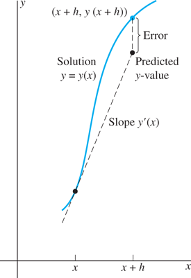
FIGURE 2.5.2.

True and predicted values in Euler’s method.

Now that $u_{n + 1} \approx y (x_{n + 1})$ $u_{n + 1} \approx y (x_{n + 1})$ has been computed, we can take

k_{2} = f (x_{n + 1}, u_{n + 1})

$k_{2} = f (x_{n + 1}, u_{n + 1})$

as a second estimate of the slope of the solution curve $y = y (x)$ $y = y (x)$ at $x = x_{n + 1}$ $x = x_{n + 1}$ .

Of course, the approximate slope $k_{1} = f (x_{n}, y_{n})$ $k_{1} = f (x_{n}, y_{n})$ at $x = x_{n}$ $x = x_{n}$ has already been calculated. Why not average these two slopes to obtain a more accurate estimate of the average slope of the solution curve over the entire subinterval $[x_{n}, x_{n + 1}] ?$ $[x_{n}, x_{n + 1}] ?$ This idea is the essence of the improved Euler method. Figure 2.5.3 shows the geometry behind this method.

FIGURE 2.5.3.

The improved Euler method: Average the slopes of the tangent lines at $(x_{n}, y_{n})$ $(x_{n}, y_{n})$ and $(x_{n + 1}, u_{n + 1}) .$ $(x_{n + 1}, u_{n + 1}) .$

Remark

The final formula in (5) takes the “Euler form”

y_{n + 1} = y_{n} + h \cdot k

$y_{n + 1} = y_{n} + h \cdot k$

if we write

k = \frac{k_{1} + k_{2}}{2}

$k = \frac{k_{1} + k_{2}}{2}$

for the approximate average slope on the interval $[x_{n}, x_{n + 1}]$ $[x_{n}, x_{n + 1}]$ .

The improved Euler method is one of a class of numerical techniques known as predictor-corrector methods. First a predictor $u_{n + 1}$ $u_{n + 1}$ of the next y-value is computed; then it is used to correct itself. Thus the improved Euler method with step size h consists of using the predictor

u_{n + 1} = y_{n} + h \cdot f (x_{n}, y_{n})

$u_{n + 1} = y_{n} + h \cdot f (x_{n}, y_{n})$ (6)

and the corrector

y_{n + 1} = y_{n} + h \cdot \frac{1}{2} [f (x_{n}, y_{n}) + f (x_{n + 1}, u_{n + 1})]

$y_{n + 1} = y_{n} + h \cdot \frac{1}{2} [f (x_{n}, y_{n}) + f (x_{n + 1}, u_{n + 1})]$ (7)

iteratively to compute successive approximations $y_{1}, y_{2}, y_{2}, \dots$ $y_{1}, y_{2}, y_{2}, \dots$ to the values $y (x_{1}), y (x_{2}), y (x_{3}), \dots$ $y (x_{1}), y (x_{2}), y (x_{3}), \dots$ of the actual solution of the initial value problem in (4).

Remark

Each improved Euler step requires two evaluations of the function f(x, y), as compared with the single function evaluation required for an ordinary Euler step. We naturally wonder whether this doubled computational labor is worth the trouble.

Answer

Under the assumption that the exact solution $y = y (x)$ $y = y (x)$ of the initial value problem in (4) has a continuous third derivative, it can be proved—see Chapter 7 of Birkhoff and Rota—that the error in the improved Euler method is of order $h^{2} .$ $h^{2} .$ This means that on a given bounded interval [a, b], each approximate value $y_{n}$ $y_{n}$ satisfies the inequality

| y (x_{n}) - y_{n} | ≦ C h^{2},

$| y (x_{n}) - y_{n} | ≦ C h^{2},$ (8)

where the constant C does not depend on h. Because $h^{2}$ $h^{2}$ is much smaller than h if h itself is small, this means that the improved Euler method is more accurate than Euler’s method itself. This advantage is offset by the fact that about twice as many computations are required. But the factor $h^{2}$ $h^{2}$ in (8) means that halving the step size results in 1/4 the maximum error, and with step size h/10 we get 100 times the accuracy (that is, 1/100 the maximum error) as with step size h.

Example 2

Figure 2.4.8 shows results of applying Euler’s method to the initial value problem

\frac{d y}{d x} = x + y, y (0) = 1

$\frac{d y}{d x} = x + y, y (0) = 1$ (9)

with exact solution $y (x) = 2 e^{x} - x - 1 .$ $y (x) = 2 e^{x} - x - 1 .$ With $f (x, y) = x + y$ $f (x, y) = x + y$ in Eqs. (6) and (7), the predictor-corrector formulas for the improved Euler method are

\begin{aligned} u_{n + 1} & = & y_{n} + h \cdot (x_{n} + y_{n}), \\ y_{n + 1} & = & y_{n} + h \cdot \frac{1}{2} [(x_{n} + y_{n}) + (x_{n + 1} + u_{n + 1})] . \end{aligned}

$\begin{aligned} u_{n + 1} & = & y_{n} + h \cdot (x_{n} + y_{n}), \\ y_{n + 1} & = & y_{n} + h \cdot \frac{1}{2} [(x_{n} + y_{n}) + (x_{n + 1} + u_{n + 1})] . \end{aligned}$

With step size $h = 0.1$ $h = 0.1$ we calculate

\begin{aligned} u_{1} & = & 1 + (0.1) \cdot (0 + 1) = 1.1, \\ y_{1} & = & 1 + (0.05) \cdot [(0 + 1) + (0.1 + 1.1)] = 1.11, \\ u_{2} & = & 1.11 + (0.1) \cdot (0.1 + 1.11) = 1.231, \\ y_{2} & = & 1.11 + (0.05) \cdot [(0.1 + 1.11) + (0.2 + 1.231)] = 1.24205, \end{aligned}

$\begin{aligned} u_{1} & = & 1 + (0.1) \cdot (0 + 1) = 1.1, \\ y_{1} & = & 1 + (0.05) \cdot [(0 + 1) + (0.1 + 1.1)] = 1.11, \\ u_{2} & = & 1.11 + (0.1) \cdot (0.1 + 1.11) = 1.231, \\ y_{2} & = & 1.11 + (0.05) \cdot [(0.1 + 1.11) + (0.2 + 1.231)] = 1.24205, \end{aligned}$

and so forth. The table in Fig. 2.5.4 compares the results obtained using the improved Euler method with those obtained previously using the “unimproved” Euler method. When the same step size $h = 0.1$ $h = 0.1$ is used, the error in the Euler approximation to y(1) is 7.25%, but the error in the improved Euler approximation is only 0.24%.

FIGURE 2.5.4.

Euler and improved Euler approximations to the solution of $d y / d x = x + y, y (0) = 1$ $d y / d x = x + y, y (0) = 1$ .

`x`	Euler Method, $h = 0.1$ $h = 0.1$ Values of `y`	Euler Method, $h = 0.005$ $h = 0.005$ Values of `y`	Improved Euler, $h = 0.1$ $h = 0.1$ Values of `y`	Actual `y`
0.1	1.1000	1.1098	1.1100	1.1103
0.2	1.2200	1.2416	1.2421	1.2428
0.3	1.3620	1.3977	1.3985	1.3997
0.4	1.5282	1.5807	1.5818	1.5836
0.5	1.7210	1.7933	1.7949	1.7974
0.6	1.9431	2.0388	2.0409	2.0442
0.7	2.1974	2.3205	2.3231	2.3275
0.8	2.4872	2.6422	2.6456	2.6511
0.9	2.8159	3.0082	3.0124	3.0192
1.0	3.1875	3.4230	3.4282	3.4366

FIGURE 2.5.5.

Improved Euler approximation to the solution of Eq. (9) with step size $h = 0.005$ $h = 0.005$ .

`x`	Improved Euler, Approximate `y`	Actual `y`
0.0	1.00000	1.00000
0.1	1.11034	1.11034
0.2	1.24280	1.24281
0.3	1.39971	1.39972
0.4	1.58364	1.58365
0.5	1.79744	1.79744
0.6	2.04423	2.04424
0.7	2.32749	2.32751
0.8	2.65107	2.65108
0.9	3.01919	3.01921
1.0	3.43654	3.43656

Indeed, the improved Euler method with $h = 0.1$ $h = 0.1$ is more accurate (in this example) than the original Euler method with $h = 0.005 .$ $h = 0.005 .$ The latter requires 200 evaluations of the function f(x, y), but the former requires only 20 such evaluations, so in this case the improved Euler method yields greater accuracy with only about one-tenth the work.

Figure 2.5.5 shows the results obtained when the improved Euler method is applied to the initial value problem in (9) using step size $h = 0.005 .$ $h = 0.005 .$ Accuracy of five significant figures is apparent in the table. This suggests that, in contrast with the original Euler method, the improved Euler method is sufficiently accurate for certain practical applications—such as plotting solution curves.

FIGURE 2.5.6.

Improved Euler approximation to y(1) for $d y / d x = - 2 x y / (1 + x^{2}), y (0) = 1.$ $d y / d x = - 2 x y / (1 + x^{2}), y (0) = 1.$

`h`	Improved Euler Approximation to `y`(1)	Error	$\| Error \| / h^{2}$ $\| Error \| / h^{2}$
0.04	0.500195903	$- 0.000195903$ $- 0.000195903$	0.12
0.02	0.500049494	$- 0.000049494$ $- 0.000049494$	0.12
0.01	0.500012437	$- 0.000012437$ $- 0.000012437$	0.12
0.005	0.500003117	$- 0.000003117$ $- 0.000003117$	0.12
0.0025	0.500000780	$- 0.000000780$ $- 0.000000780$	0.12
0.00125	0.500000195	$- 0.000000195$ $- 0.000000195$	0.12
0.000625	0.500000049	$- 0.000000049$ $- 0.000000049$	0.12
0.0003125	0.500000012	$- 0.000000012$ $- 0.000000012$	0.12

An improved Euler program (similar to the ones listed in the project material for this section) was used to compute approximations to the exact value $y (1) = 0.5$ $y (1) = 0.5$ of the solution $y (x) = 1 / (1 + x^{2})$ $y (x) = 1 / (1 + x^{2})$ of the initial value problem

\frac{d y}{d x} = - \frac{2 x y}{1 + x^{2}}, y (0) = 1

$\frac{d y}{d x} = - \frac{2 x y}{1 + x^{2}}, y (0) = 1$ (3)

of Example 1. The results obtained by successively halving the step size appear in the table in Fig. 2.5.6. Note that the final column of this table impressively corroborates the form of the error bound in (8), and that each halving of the step size reduces the error by a factor of almost exactly 4, as should happen if the error is proportional to $h^{2} .$ $h^{2} .$

In the following two examples we exhibit graphical results obtained by employing this strategy of successively halving the step size, and thus doubling the number of subintervals of a fixed interval on which we are approximating a solution.

Example 3

In Example 3 of Section 2.4 we applied Euler’s method to the logistic initial value problem

\frac{d y}{d x} = \frac{1}{3} y (8 - y), y (0) = 1.

$\frac{d y}{d x} = \frac{1}{3} y (8 - y), y (0) = 1.$

Figure 2.4.9 shows an obvious difference between the exact solution $y (x) =$ $y (x) =$ $8 / (1 + 7 e^{- 8 x / 3})$ $8 / (1 + 7 e^{- 8 x / 3})$ and the Euler approximation on $0 ≦ x ≦ 5$ $0 ≦ x ≦ 5$ using $n = 20$ $n = 20$ subintervals. Figure 2.5.7 shows approximate solution curves plotted using the improved Euler’s method.

The approximation with five subintervals is still bad—perhaps worse! It appears to level off considerably short of the actual limiting population $M = 8 .$ $M = 8 .$ You should carry out at least the first two improved Euler steps manually to see for yourself how it happens that, after increasing appropriately during the first step, the approximate solution decreases in the second step rather than continuing to increase (as it should). In the project for this section we ask you to show empirically that the improved Euler approximate solution with step size $h = 1$ $h = 1$ levels off at $y \approx 4.3542$ $y \approx 4.3542$ .

In contrast, the approximate solution curve with $n = 20$ $n = 20$ subintervals tracks the exact solution curve rather closely, and with $n = 40$ $n = 40$ subintervals the exact and approximate solution curves are indistinguishable in Fig. 2.5.7. The table in Fig. 2.5.8 indicates that the improved Euler approximation with $n = 200$ $n = 200$ subintervals is accurate rounded to three decimal places (that is, four significant digits) on the interval $0 ≦ x ≦ 5 .$ $0 ≦ x ≦ 5 .$ Because discrepancies in the fourth significant digit are not visually apparent at the resolution of an ordinary computer screen, the improved Euler method (using several hundred subintervals) is considered adequate for many graphical purposes.

FIGURE 2.5.7.

Approximating a logistic solution using the improved Euler method with $n = 5, n = 10, n = 20,$ $n = 5, n = 10, n = 20,$ and $n = 40$ $n = 40$ subintervals.

FIGURE 2.5.8.

Using the improved Euler method to approximate the actual solution of the initial value problem in Example 3.

`x`	Actual `y`(`x`)	Improved Euler with $n = 200$ $n = 200$
0	1.0000	1.0000
1	5.3822	5.3809
2	7.7385	7.7379
3	7.9813	7.9812
4	7.9987	7.9987
5	7.9999	7.9999

Example 4

In Example 4 of Section 2.4 we applied Euler’s method to the initial value problem

\frac{d y}{d x} = y \cos x, y (0) = 1.

$\frac{d y}{d x} = y \cos x, y (0) = 1.$

Figure 2.4.10 shows obvious visual differences between the periodic exact solution $y (x) = e^{\sin x}$ $y (x) = e^{\sin x}$ and the Euler approximations on $0 ≦ x ≦ 6 π$ $0 ≦ x ≦ 6 π$ with as many as $n = 400$ $n = 400$ subintervals.

FIGURE 2.5.9.

Approximating the exact solution $y = e^{\sin x}$ $y = e^{\sin x}$ using the improved Euler method with $n = 50,$ $n = 50,$ 100, and 200 subintervals.

Figure 2.5.9 shows the exact solution curve and approximate solution curves plotted using the improved Euler method with $n = 50, n = 100,$ $n = 50, n = 100,$ and $n = 200$ $n = 200$ subintervals. The approximation obtained with $n = 200$ $n = 200$ is indistinguishable from the exact solution curve, and the approximation with $n = 100$ $n = 100$ is only barely distinguishable from it.

Although Figs. 2.5.7 and 2.5.9 indicate that the improved Euler method can provide accuracy that suffices for many graphical purposes, it does not provide the higher-precision numerical accuracy that sometimes is needed for more careful investigations. For instance, consider again the initial value problem

\frac{d y}{d x} = - \frac{2 x y}{1 + x^{2}}, y (0) = 1

$\frac{d y}{d x} = - \frac{2 x y}{1 + x^{2}}, y (0) = 1$

of Example 1. The final column of the table in Fig. 2.5.6 suggests that, if the improved Euler method is used on the interval $0 ≦ x ≦ 1$ $0 ≦ x ≦ 1$ with n subintervals and step size $h = 1 / n,$ $h = 1 / n,$ then the resulting error E in the final approximation $y_{n} \approx y (1)$ $y_{n} \approx y (1)$ is given by

E = | y (1) - y_{n} | \approx (0.12) h^{2} = \frac{0.12}{n^{2}} .

$E = | y (1) - y_{n} | \approx (0.12) h^{2} = \frac{0.12}{n^{2}} .$

If so, then 12-place accuracy (for instance) in the value y(1) would require that $(0.12) n^{- 2} < 5 \times 10^{- 13},$ $(0.12) n^{- 2} < 5 \times 10^{- 13},$ which means that $n ≧ 489, 898 .$ $n ≧ 489, 898 .$ Thus, roughly half a million steps of length $h \approx 0.000002$ $h \approx 0.000002$ would be required. Aside from the possible impracticality of this many steps (using available computational resources), the roundoff error resulting from so many successive steps might well overwhelm the cumulative error predicted by theory (which assumes exact computations in each separate step). Consequently, still more accurate methods than the improved Euler method are needed for such high-precision computations. Such a method is presented in Section 2.6.

2.5 Problems

A hand-held calculator will suffice for Problems 1 through 10, where an initial value problem and its exact solution are given. Apply the improved Euler method to approximate this solution on the interval [0, 0.5] with step size $h = 0.1 .$ $h = 0.1 .$ Construct a table showing four-decimal-place values of the approximate solution and actual solution at the points $x = 0.1, 0.2, 0.3, 0.4, 0.5$ $x = 0.1, 0.2, 0.3, 0.4, 0.5$ .

$y ′ = - y,$ $y ′ = - y,$ $y (0) = 2;$ $y (0) = 2;$ $y (x) = 2 e^{- x}$ $y (x) = 2 e^{- x}$
$y ′ = 2 y,$ $y ′ = 2 y,$ $y (0) = \frac{1}{2};$ $y (0) = \frac{1}{2};$ $y (x) = \frac{1}{2} e^{2 x}$ $y (x) = \frac{1}{2} e^{2 x}$
$y ′ = y + 1,$ $y ′ = y + 1,$ $y (0) = 1;$ $y (0) = 1;$ $y (x) = 2 e^{x} - 1$ $y (x) = 2 e^{x} - 1$
$y ′ = x - y,$ $y ′ = x - y,$ $y (0) = 1;$ $y (0) = 1;$ $y (x) = 2 e^{- x} + x - 1$ $y (x) = 2 e^{- x} + x - 1$
$y ′ = y - x - 1,$ $y ′ = y - x - 1,$ $y (0) = 1;$ $y (0) = 1;$ $y (x) = 2 + x - e^{x}$ $y (x) = 2 + x - e^{x}$
$y ′ = - 2 x y,$ $y ′ = - 2 x y,$ $y (0) = 2;$ $y (0) = 2;$ $y (x) = 2 e^{- x^{2}}$ $y (x) = 2 e^{- x^{2}}$
$y ′ = - 3 x^{2} y,$ $y ′ = - 3 x^{2} y,$ $y (0) = 3;$ $y (0) = 3;$ $y (x) = 3 e^{- x^{3}}$ $y (x) = 3 e^{- x^{3}}$
$y ′ = e^{- y},$ $y ′ = e^{- y},$ $y (0) = 0;$ $y (0) = 0;$ $y (x) = \ln (x + 1)$ $y (x) = \ln (x + 1)$
$y ′ = \frac{1}{4} (1 + y^{2}),$ $y ′ = \frac{1}{4} (1 + y^{2}),$ $y (0) = 1;$ $y (0) = 1;$ $y (x) = \tan \frac{1}{4} (x + π)$ $y (x) = \tan \frac{1}{4} (x + π)$
$y ′ = 2 {x y}^{2},$ $y ′ = 2 {x y}^{2},$ $y (0) = 1;$ $y (0) = 1;$ $y (x) = \frac{1}{1 - x^{2}}$ $y (x) = \frac{1}{1 - x^{2}}$

Note: The application following this problem set lists illustrative calculator/computer programs that can be used in Problems 11 through 24.

A programmable calculator or a computer will be useful for Problems 11 through 16. In each problem find the exact solution of the given initial value problem. Then apply the improved Euler method twice to approximate (to five decimal places) this solution on the given interval, first with step size $h = 0.01,$ $h = 0.01,$ then with step size $h = 0.005 .$ $h = 0.005 .$ Make a table showing the approximate values and the actual value, together with the percentage error in the more accurate approximations, for x an integral multiple of 0.2. Throughout, primes denote derivatives with respect to x.

$y ′ = y - 2,$ $y ′ = y - 2,$ $y (0) = 1;$ $y (0) = 1;$ $0 ≦ x ≦ 1$ $0 ≦ x ≦ 1$
$y ′ = \frac{1}{2} {(y - 1)}^{2},$ $y ′ = \frac{1}{2} {(y - 1)}^{2},$ $y (0) = 2;$ $y (0) = 2;$ $0 ≦ x ≦ 1$ $0 ≦ x ≦ 1$
$y y ′ = 2 x^{3},$ $y y ′ = 2 x^{3},$ $y (1) = 3;$ $y (1) = 3;$ $1 ≦ x ≦ 2$ $1 ≦ x ≦ 2$
$x y ′ = y^{2},$ $x y ′ = y^{2},$ $y (1) = 1;$ $y (1) = 1;$ $1 ≦ x ≦ 2$ $1 ≦ x ≦ 2$
$x y ′ = 3 x - 2 y,$ $x y ′ = 3 x - 2 y,$ $y (2) = 3;$ $y (2) = 3;$ $2 ≦ x ≦ 3$ $2 ≦ x ≦ 3$
$y^{2} y ′ = 2 x^{5},$ $y^{2} y ′ = 2 x^{5},$ $y (2) = 3;$ $y (2) = 3;$ $2 ≦ x ≦ 3$ $2 ≦ x ≦ 3$

A computer with a printer is required for Problems 17 through 24. In these initial value problems, use the improved Euler method with step sizes $h = 0.1, 0.02, 0.004,$ $h = 0.1, 0.02, 0.004,$ and 0.0008 to approximate to five decimal places the values of the solution at ten equally spaced points of the given interval. Print the results in tabular form with appropriate headings to make it easy to gauge the effect of varying the step size h. Throughout, primes denote derivatives with respect to x.

$y ′ = x^{2} + y^{2},$ $y ′ = x^{2} + y^{2},$ $y (0) = 0;$ $y (0) = 0;$ $0 ≦ x ≦ 1$ $0 ≦ x ≦ 1$
$y ′ = x^{2} - y^{2},$ $y ′ = x^{2} - y^{2},$ $y (0) = 1;$ $y (0) = 1;$ $0 ≦ x ≦ 2$ $0 ≦ x ≦ 2$
$y ′ = x + \sqrt{y},$ $y ′ = x + \sqrt{y},$ $y (0) = 1;$ $y (0) = 1;$ $0 ≦ x ≦ 2$ $0 ≦ x ≦ 2$
$y ′ = x + \sqrt[3]{y},$ $y ′ = x + \sqrt[3]{y},$ $y (0) = - 1;$ $y (0) = - 1;$ $0 ≦ x ≦ 2$ $0 ≦ x ≦ 2$
$y ′ = \ln y,$ $y ′ = \ln y,$ $y (1) = 2;$ $y (1) = 2;$ $1 ≦ x ≦ 2$ $1 ≦ x ≦ 2$
$y ′ = x^{2/3} + y^{2/3},$ $y ′ = x^{2/3} + y^{2/3},$ $y (0) = 1;$ $y (0) = 1;$ $0 ≦ x ≦ 2$ $0 ≦ x ≦ 2$
$y ′ = \sin x + \cos y,$ $y ′ = \sin x + \cos y,$ $y (0) = 0;$ $y (0) = 0;$ $0 ≦ x ≦ 1$ $0 ≦ x ≦ 1$
$y ′ = \frac{x}{1 + y^{2}},$ $y ′ = \frac{x}{1 + y^{2}},$ $y (- 1) = 1;$ $y (- 1) = 1;$ $- 1 ≦ x ≦ 1$ $- 1 ≦ x ≦ 1$
Falling parachutist As in Problem 25 of Section 2.4, you bail out of a helicopter and immediately open your parachute, so your downward velocity satisfies the initial value problem

$\frac{d v}{d t} = 32 - 1.6 v, v (0) = 0$ $\frac{d v}{d t} = 32 - 1.6 v, v (0) = 0$

(with t in seconds and v in ft/s). Use the improved Euler method with a programmable calculator or computer to approximate the solution for $0 ≦ t ≦ 2,$ $0 ≦ t ≦ 2,$ first with step size $h = 0.01$ $h = 0.01$ and then with $h = 0.005,$ $h = 0.005,$ rounding off approximate v-values to three decimal places. What percentage of the limiting velocity 20 ft/s has been attained after 1 second? After 2 seconds?
Deer population As in Problem 26 of Section 2.4, suppose the deer population P(t) in a small forest initially numbers 25 and satisfies the logistic equation

$\frac{d P}{d t} = 0.0225 P - 0.0003 P^{2}$ $\frac{d P}{d t} = 0.0225 P - 0.0003 P^{2}$

(with t in months). Use the improved Euler method with a programmable calculator or computer to approximate the solution for 10 years, first with step size $h = 1$ $h = 1$ and then with $h = 0.5,$ $h = 0.5,$ rounding off approximate P-values to three decimal places. What percentage of the limiting population of 75 deer has been attained after 5 years? After 10 years?

Decreasing Step Size

Use the improved Euler method with a computer system to find the desired solution values in Problems 27 and 28. Start with step size $h = 0.1,$ $h = 0.1,$ and then use successively smaller step sizes until successive approximate solution values at $x = 2$ $x = 2$ agree rounded off to four decimal places.

$y ′ = x^{2} + y^{2} - 1, y (0) = 0;$ $y ′ = x^{2} + y^{2} - 1, y (0) = 0;$ $y (2) = ?$ $y (2) = ?$
$y ′ = x + \frac{1}{2} y^{2}, y (- 2) = 0;$ $y ′ = x + \frac{1}{2} y^{2}, y (- 2) = 0;$ $y (2) = ?$ $y (2) = ?$
Velocity-proportional resistance Consider the crossbow bolt of Example 2 in Section 2.3, shot straight upward from the ground with an initial velocity of 49 m/s. Because of linear air resistance, its velocity function v(t) satisfies the initial value problem

$\begin{array}{l} \frac{d υ}{d t} = - (0.04) υ - 9.8, & υ (0) = 49 \end{array}$ $\begin{array}{l} \frac{d υ}{d t} = - (0.04) υ - 9.8, & υ (0) = 49 \end{array}$

with exact solution $v (t) = 294 e^{- t / 25} - 245 .$ $v (t) = 294 e^{- t / 25} - 245 .$ Use a calculator or computer implementation of the improved Euler method to approximate v(t) for $0 ≦ t ≦ 10$ $0 ≦ t ≦ 10$ using both $n = 50$ $n = 50$ and $n = 100$ $n = 100$ subintervals. Display the results at intervals of 1 second. Do the two approximations—each rounded to two decimal places—agree both with each other and with the exact solution? If the exact solution were unavailable, explain how you could use the improved Euler method to approximate closely (a) the bolt’s time of ascent to its apex (given in Section 2.3 as 4.56 s) and (b) its impact velocity after 9.41 s in the air.
Square-proportional resistance Consider now the crossbow bolt of Example 3 in Section 2.3. It still is shot straight upward from the ground with an initial velocity of 49 m/s, but because of air resistance proportional to the square of its velocity, its velocity function v(t) satisfies the initial value problem

$\frac{d v}{d t} = - (0.0011) v | v | - 9.8, v (0) = 49.$ $\frac{d v}{d t} = - (0.0011) v | v | - 9.8, v (0) = 49.$

The symbolic solution discussed in Section 2.3 required separate investigations of the bolt’s ascent and its descent, with v(t) given by a tangent function during ascent and by a hyperbolic tangent function during descent. But the improved Euler method requires no such distinction. Use a calculator or computer implementation of the improved Euler method to approximate v(t) for $0 ≦ t ≦ 10$ $0 ≦ t ≦ 10$ using both $n = 100$ $n = 100$ and $n = 200$ $n = 200$ subintervals. Display the results at intervals of 1 second. Do the two approximations—each rounded to two decimal places—agree with each other? If an exact solution were unavailable, explain how you could use the improved Euler method to approximate closely (a) the bolt’s time of ascent to its apex (given in Section 2.3 as 4.61 s) and (b) its impact velocity after 9.41 s in the air.

2.5 Application Improved Euler Implementation

Figure 2.5.10 lists TI-84 Plus and Python programs implementing the improved Euler method to approximate the solution of the initial value problem

\frac{d y}{d x} = x + y, y (0) = 1

$\frac{d y}{d x} = x + y, y (0) = 1$

considered in Example 2 of this section. The comments provided in the final column should make these programs intelligible even if you have little familiarity with the Python and TI programming languages.

To apply the improved Euler method to a differential equation $d y / d x = f (x, y),$ $d y / d x = f (x, y),$ one need only replace x+y throughout with the desired expression. To increase the number of steps (and thereby decrease the step size) one need only change the value of N specified in the second line of the program.

FIGURE 2.5.10.

TI-84 Plus and Python improved Euler programs.

TI-84 Plus	Python	Comment
`PROGRAM: IMPEULER`	`# Program IMPEULER`	`Program title`
	`def F(X,Y): return X + Y`	`Define function f`
`:10→N`	`N = 10`	`No. of steps`
`:0→X`	`X = 0.0`	`Initial x`
`:1→Y`	`Y = 1.0`	`Initial y`
`:1→T`	`X1 = 1.0`	`Final x`
`:(T-X)/N→H`	`H = (X1-X)/N`	`Step size`
`:For(I,1,N)`	`for I in range(N):`	`Begin loop`
`:Y→Z`	`Y0 = Y`	`Save previous y`
`:X+Y→K`	`K1 = F(X,Y)`	`First slope`
`:Z+H*K→Y`	`Y = Y0 + H*K1`	`Predictor`
`:X+H→X`	`X = X + H`	`New x`
`:X+Y→L`	`K2 = F(X,Y)`	`Second slope`
`:(K+L)/2→K`	`K = (K1 + K2)/2`	`Average slope`
`:Z+H*K→Y`	`Y = Y0 + H*K`	`Corrector`
`:Disp X,Y`	`print (X,Y)`	`Display results`
`:End`	`# END`	`End loop`

Figure 2.5.11 exhibits one Matlab implementation of the improved Euler method. The impeuler function takes as input the initial value x, the initial value y, the final value x1 of x, and the desired number n of subintervals. As output it produces the resulting column vectors x and y of x- and y-values. For instance, the Matlab command

[X, Y] = impeuler(0, 1, 1, 10)

then generates the first and fourth columns of data shown in Fig. 2.5.4.

function yp = f(x,y)
yp = x + y;                   % yp = y’
function [X,Y] = impeuler(x,y,x1,n)
h = (x1 - x)/n;               % step size
X = x;                        % initial x
Y = y;                        % initial y
for i = 1:n;                  % begin loop
    k1 = f(x,y);              % first slope
    k2 = f(x+h,y+h*k1);       % second slope
    k = (k1 + k2)/2;;         % average slope
    x = x + h;                % new x
    y = y + h*k;              % new y
    X = [X;x];                % update x-column
    Y = [Y;y];                % update y-column
    end                       % end loop

FIGURE 2.5.11.

Matlab implementation of improved Euler method.

You should begin this project by implementing the improved Euler method with your own calculator or computer system. Test your program by applying it first to the initial value problem of Example 1, then to some of the problems for this section.

Famous Numbers Revisited

The following problems describe the numbers $e \approx 2.7182818, \ln 2 \approx 0.6931472,$ $e \approx 2.7182818, \ln 2 \approx 0.6931472,$ and $π \approx 3.1415927$ $π \approx 3.1415927$ as specific values of certain initial value problems. In each case, apply the improved Euler method with $n = 10, 20, 40, \dots$ $n = 10, 20, 40, \dots$ subintervals (doubling n each time). How many subintervals are needed to obtain—twice in succession—the correct value of the target number rounded to five decimal places?

The number $e = y (1),$ $e = y (1),$ where y(x) is the solution of the initial value problem $d y / d x = y, y (0) = 1$ $d y / d x = y, y (0) = 1$ .
The number $\ln 2 = y (2),$ $\ln 2 = y (2),$ where y(x) is the solution of the initial value problem $d y / d x = 1 / x, y (1) = 0$ $d y / d x = 1 / x, y (1) = 0$ .
The number $π = y (1),$ $π = y (1),$ where y(x) is the solution of the initial value problem $d y / d x = 4 / (1 + x^{2}), y (0) = 0$ $d y / d x = 4 / (1 + x^{2}), y (0) = 0$ .

Logistic Population Investigation

Apply your improved Euler program to the initial value problem $d y / d x = \frac{1}{3} y (8 - y), y (0) = 1$ $d y / d x = \frac{1}{3} y (8 - y), y (0) = 1$ of Example 3. In particular, verify (as claimed) that the approximate solution with step size $h = 1$ $h = 1$ levels off at $y \approx 4.3542$ $y \approx 4.3542$ rather than at the limiting value $y = 8$ $y = 8$ of the exact solution. Perhaps a table of values for $0 ≦ x ≦ 100$ $0 ≦ x ≦ 100$ will make this apparent.

For your own logistic population to investigate, consider the initial value problem

\frac{d y}{d x} = \frac{1}{n} y (m - y), y (0) = 1

$\frac{d y}{d x} = \frac{1}{n} y (m - y), y (0) = 1$

where m and n are (for instance) the largest and smallest nonzero digits in your student ID number. Does the improved Euler approximation with step size $h = 1$ $h = 1$ level off at the “correct” limiting value of the exact solution? If not, find a smaller value of h so that it does.

Periodic Harvesting and Restocking

The differential equation

\frac{d y}{d t} = k y (M - y) - h \sin (\frac{2 π t}{P})

$\frac{d y}{d t} = k y (M - y) - h \sin (\frac{2 π t}{P})$

models a logistic population that is periodically harvested and restocked with period P and maximal harvesting/restocking rate h. A numerical approximation program was used to plot the typical solution curves for the case $k = M = h = P = 1$ $k = M = h = P = 1$ that are shown in Fig. 2.5.12. This figure suggests—although it does not prove—the existence of a threshold initial population such that

FIGURE 2.5.12.

Solution curves of $d y / d t = y (1 - y) - \sin 2 π t$ $d y / d t = y (1 - y) - \sin 2 π t$ .

Beginning with an initial population above this threshold, the population oscillates (perhaps with period P?) around the (unharvested) stable limiting population $y (t) \equiv M,$ $y (t) \equiv M,$ whereas
The population dies out if it begins with an initial population below this threshold.

Use an appropriate plotting utility to investigate your own logistic population with periodic harvesting and restocking (selecting typical values of the parameters k, M, h, and P). Do the observations indicated here appear to hold for your population?

..................Content has been hidden....................

You can't read the all page of ebook, please click here login for view all page.

Table of Contents for An Improvement in Euler’s Method

Create new playlist

Sign In

Sign Up

Table of Contents for
An Improvement in Euler’s Method