
9.4 Nonlinear Mechanical Systems
Now we apply the qualitative methods of Sections 9.1 and 9.2 to the analysis of simple mechanical systems like the mass-on-a-spring system shown in Fig. 9.4.1. Let m denote the mass in a suitable system of units and let x(t) denote the displacement of the mass at time t from its equilibrium position (in which the spring is unstretched). Previously we have always assumed that the force F(x) exerted by the spring on the mass is a linear function of x: F(x)=−kx

FIGURE 9.4.1.
The mass on a spring.
So now we allow the force function F(x) to be nonlinear. Because F(0)=0
We take k>0
For a simple mathematical model of a nonlinear spring we therefore take
![]()
ignoring all terms in Eq. (1) of degree greater than 3. The equation of motion of the mass m is then
![]()
The Position–Velocity Phase Plane
If we introduce the velocity
of the mass with position x(t), then we get from Eq. (3) the equivalent first-order system
A phase plane trajectory of this system is a position-velocity plot that illustrates the motion of the mass on the spring. We can solve explicitly for the trajectories of this system by writing
whence
Integration then yields
for the equation of a typical trajectory. We write E for the arbitrary constant of integration because KE=12my2
as the potential energy of the spring. Then Eq. (6) takes the form KE+PE=E,
The behavior of the mass depends on the sign of the nonlinear term in Eq. (2). The spring is called
hard if β<0
β<0 ,soft if β>0
β>0 .
We consider the two cases separately.
Hard Spring Oscillations: If β<0,
is an oval closed curve like those shown in Fig. 9.4.2, and thus (0, 0) is a stable center. As the point (x(t), y(t)) traverses a trajectory in the clockwise direction, the position x(t) and velocity y(t) of the mass oscillate alternately, as illustrated in Fig. 9.4.3. The mass is moving to the right (with x increasing) when y>0,
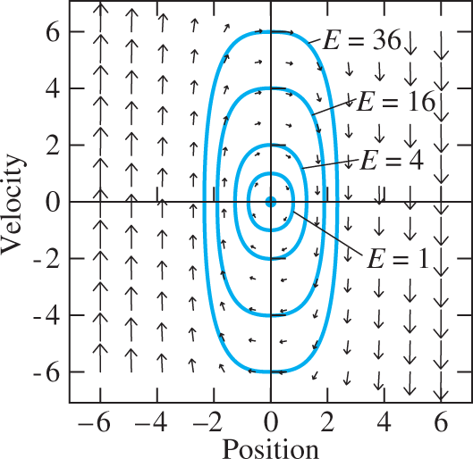
FIGURE 9.4.2.
Position-velocity phase plane portrait for the hard mass-and-spring system with m=k=2

FIGURE 9.4.3.
Position and velocity solution curves for the hard mass-and-spring system with m=k=2
Remark
The hard spring equation mx″=−kx−|β|x3
with Jacobian matrix
(writing k/m=ω2
Soft Spring Oscillations: If β>0,
Example 1
Undamped soft spring If m=1, k=4,
and Eq. (6) gives the trajectories in the form
After solving for
we could select a fixed value of the constant energy E and plot manually a trajectory like one of those shown in the computer-generated position-velocity phase plane portrait in Fig. 9.4.4.
The different types of phase plane trajectories correspond to different values of the energy E. If we substitute x=±√k/β
The nature of the motion of the mass is determined by which type of trajectory its initial conditions determine. The simple closed trajectories encircling (0, 0) in the region bounded by the separatrices correspond to energies in the range 0<E<4.
The unbounded trajectories lying in the regions above and below the separatrices correspond to values of E greater than 4. These represent motions in which the mass approaches x=0

FIGURE 9.4.4.
Position–velocity phase plane portrait for the soft mass-and-spring system with m=1,k=4,

FIGURE 9.4.5.
Position and velocity solution curves for the soft mass-and-spring system with m=1,k=4,β=1>0,
The unbounded trajectories opening to the right and left correspond to values of E less than 4. These represent motions in which the mass initially is headed toward the equilibrium point x=0,
In Fig. 9.4.4 it appears that the critical point (0, 0) is a stable center, whereas the critical points (±2,0)
with Jacobian matrix
To check these observations against the usual critical-point analysis, we note first that the Jacobian matrix
at the critical point (0, 0) has characteristic equation λ2+4=0
corresponding to the other two critical points has characteristic equation λ2−8=0
Remark
Figures 9.4.2 and 9.4.4 illustrate a significant qualitative difference between hard springs with β<0
Damped Nonlinear Vibrations
Suppose now that the mass on a spring is connected also to a dashpot that provides a force of resistance proportional to the velocity y=dx/dt
![]()
where c>0
has critical points (0, 0) and (±√k/β,0)
Now the critical point at the origin is the most interesting one. The Jacobian matrix
has characteristic equation
and eigenvalues
It follows from Theorem 2 in Section 9.2 in that the critical point (0, 0) of the system in (13) is
a nodal sink if the resistance is so great that c2>4km
c2>4km (in which case the eigenvalues are negative and unequal), but isa spiral sink if c2<4km
c2<4km (in which case the eigenvalues are complex conjugates with negative real part).
The following example illustrates the latter case. (In the borderline case with equal negative eigenvalues, the origin may be either a nodal or a spiral sink.)
Example 2
Damped soft spring Suppose that m=1, c=2, k=5,
It has critical points (0,0), (±2,0)
At (0, 0): The Jacobian matrix
has characteristic equation λ2+2λ+5=0
that corresponds to an exponentially damped oscillation about the equilibrium position x=0
At (±2,0)
has characteristic equation λ2+2λ−10=0
The position–velocity phase plane portrait in Fig. 9.4.6 shows trajectories of (14) and the spiral sink at (0, 0), as well as the unstable saddle points at (−2,0)
Region I between the separatrices, then the trajectory spirals into the origin as t→+∞,
t→+∞, and hence the periodic oscillations of the undamped case (Fig. 9.4.4) are now replaced with damped oscillations around the stable equilibrium position x=0x=0 ;Region II, then the mass passes through x=0
x=0 moving from left to right (x increasing);Region III, then the mass passes through x=0
x=0 moving from right to left (x decreasing);Region IV, then the mass approaches (but does not reach) the unstable equilibrium position x=−2
x=−2 from the left, but stops and then returns to the left;Region V, then the mass approaches (but does not reach) the unstable equilibrium position x=2
x=2 from the right, but stops and then returns to the right.

FIGURE 9.4.6.
Position–velocity phase plane portrait for the soft mass-and-spring system with m=1,k=5,β=54,
If the initial point (x0,y0)
The Nonlinear Pendulum
In Section 5.4 we derived the equation
![]()
for the undamped oscillations of the simple pendulum shown in Fig. 9.4.7. There we used the approximation sin θ≈θ
where ω2=g/L.
of Eq. (16) describes oscillations around the equilibrium position θ=0

FIGURE 9.4.7.
The simple pendulum.
The linear model does not adequately describe the possible motions of the pendulum for large values of θ.
![]()
The case c>0
We see that this system is almost linear by writing it in the form
where
has only higher-degree terms.
The critical points of the system in (19) are the points (nπ,0)
The nature of the critical point (nπ,0)
Even Case: If n=2m
with characteristic equation λ2+ω2=0
for which (0, 0) is the familiar stable center enclosed by elliptical trajectories (as in Example 3 of Section 9.1). Although this is the delicate case for which Theorem 2 of Section 9.2 does not settle the matter, we will see presently that (2mπ,0)
Odd Case: If n=2m+1
with characteristic equation λ2−ω2=0
for which (0, 0) is a saddle point. It follows from Theorem 2 of Section 9.2 that the critical point ((2m+1)π,0)
The Trajectories: We can see how these “even centers” and “odd saddle points” fit together by solving the system in (19) explicitly for the phase plane trajectories. If we write
and separate the variables,
then integration from x=0
We write E for the arbitrary constant of integration because, if physical units are so chosen that m=L=1,
If we solve Eq. (24) for y and use a half-angle identity, we get the equation
that defines the phase plane trajectories. Note that the radicand in (25) remains positive if E>2ω2.

FIGURE 9.4.8.
Position–velocity phase plane portrait for the undamped pendulum system x′=y,y′=−sinx.
The emphasized separatrices in Fig. 9.4.8 correspond to the critical value E=2ω2
The simple closed trajectories encircling the stable critical points—all of which correspond to the downward position θ=2mπ
The unbounded trajectories with E>2ω2
Period of Undamped Oscillation
If the pendulum is released from rest with initial conditions
then Eq. (24) with t=0
Hence E<2ω2
The period T of time required for one complete oscillation is four times the amount of time required for θ
To attempt to evaluate this integral we first use the identity cos θ=1−2sin2(θ/2)
where
Next, the substitution u=(1/k)sin(θ/2)
Finally, the substitution u=sin ϕ
The integral in (30) is the elliptic integral of the first kind that is often denoted by F(k,π/2).
with x=k2 sin2 ϕ<1
The final result is the formula
for the period T of the nonlinear pendulum released from rest with initial angle θ(0)=α,
The infinite series within the second pair of brackets in Eq. (33) gives the factor T/T0
shows that the linearized model is quite inadequate for a pendulum clock; a discrepancy of 19 min 9 s after only one week is unacceptable.
FIGURE 9.4.9.
Dependence of the period T of a nonlinear pendulum on its initial angle α
| α |
T/T0 |
|---|---|
| 10° |
1.0019 |
| 20° |
1.0077 |
| 30° |
1.0174 |
| 40° |
1.0313 |
| 50° |
1.0498 |
| 60° |
1.0732 |
| 70° |
1.1021 |
| 80° |
1.1375 |
| 90° |
1.1803 |
Damped Pendulum Oscillations
Finally, we discuss briefly the damped nonlinear pendulum. The almost linear first-order system equivalent to Eq. (19) is
and again the critical points are of the form (nπ,0)
If n is odd, then (nπ,0)
(nπ,0) is an unstable saddle point of (34), just as in the undamped case; butIf n is even and c2>4ω2,
c2>4ω2, then (nπ,0)(nπ,0) is a nodal sink; whereasIf n is even and c2<4ω2,
c2<4ω2, then (nπ,0)(nπ,0) is a spiral sink.
Figure 9.4.10 illustrates the phase plane trajectories for the more interesting underdamped case, c2<4ω2.

FIGURE 9.4.10.
Position–velocity phase plane portrait for the damped pendulum system x′=y,y′=−sinx−14y.
9.4 Problems
In Problems 1 through 4, show that the given system is almost linear with (0, 0) as a critical point, and classify this critical point as to type and stability. Use a computer system or graphing calculator to construct a phase plane portrait that illustrates your conclusion.
dxdt=1−ex+2y, dydt=−x−4sin y
dxdt=1−ex+2y, dydt=−x−4sin y dxdt=2sin x+sin y, dydt=sin x+2sin y
dxdt=2sin x+sin y, dydt=sin x+2sin y (Fig. 9.4.11)
FIGURE 9.4.11.
Trajectories of the system in Problem 2.
dxdt=ex+2y−1, dydt=8x+ey−1
dxdt=ex+2y−1, dydt=8x+ey−1 dxdt=sin xcos y−2y, dydt=4x−3cos xsin y
dxdt=sin xcos y−2y, dydt=4x−3cos xsin y
Find and classify each of the critical points of the almost linear systems in Problems 5 through 8. Use a computer system or graphing calculator to construct a phase plane portrait that illustrates your findings.
dxdt=−x+sin y, dydt=2x
dxdt=−x+sin y, dydt=2x dxdt=y, dydt=sin πx−y
dxdt=y, dydt=sin πx−y dxdt=1−ex−y, dydt=2sin x
dxdt=1−ex−y, dydt=2sin x dxdt=3sin x+y, dydt=sin x+2y
dxdt=3sin x+y, dydt=sin x+2y
Critical Points for Damped Pendulum
Problems 9 through 11 deal with the damped pendulum system x′=y, y′=−ω2 sin x−cy
Show that if n is an odd integer, then the critical point (nπ,0)
(nπ,0) is a saddle point for the damped pendulum system.Show that if n is an even integer and c2>4ω2,
c2>4ω2, then the critical point (nπ,0)(nπ,0) is a nodal sink for the damped pendulum system.Show that if n is an even integer and c2<4ω2,
c2<4ω2, then the critical point (nπ,0)(nπ,0) is a spiral sink for the damped pendulum system.
Critical Points for Mass-Spring System
In each of Problems 12 through 16, a second-order equation of the form x″+f(x,x′)=0,
x″+20x−5x3=0
x''+20x−5x3=0 : Verify that the critical points resemble those shown in Fig. 9.4.4.x″+2x′+20x−5x3=0
x''+2x'+20x−5x3=0 : Verify that the critical points resemble those shown in Fig. 9.4.6.x″−8x+2x3=0
x''−8x+2x3=0 : Here the linear part of the force is repulsive rather than attractive (as for an ordinary spring). Verify that the critical points resemble those shown in Fig. 9.4.12. Thus there are two stable equilibrium points and three types of periodic oscillations.x″+4x−x2=0
x''+4x−x2=0 : Here the force function is nonsymmetric. Verify that the critical points resemble those shown in Fig. 9.4.13.x″+4x−5x3+x5=0
x''+4x−5x3+x5=0 : The idea here is that terms through the fifth degree in an odd force function have been retained. Verify that the critical points resemble those shown in Fig. 9.4.14.
Critical Points for Physical Systems
In Problems 17 through 20, analyze the critical points of the indicated system, use a computer system to construct an illustrative position–velocity phase plane portrait, and describe the oscillations that occur.
Example 2 illustrates the case of damped vibrations of a soft mass–spring system with the resistance proportional to the velocity. Investigate an example of resistance proportional to the square of the velocity by using the same parameters as in Example 2, but with resistance term −cx′|x′|
−cx'|x'| instead of −cx′−cx' in Eq. (12).The equations x′=y, y′=−sin x−14y|y|
x'=y, y'=−sin x−14y∣∣y∣∣ model a damped pendulum system as in Eqs. (34) and Fig. 9.4.10. But now the resistance is proportional to the square of the angular velocity of the pendulum. Compare the oscillations with those that occur when the resistance is proportional to the angular velocity itself.
Period of Oscillation
Problems 21 through 26 outline an investigation of the period T of oscillation of a mass on a nonlinear spring with equation of motion
If ϕ(x)=kx

FIGURE 9.4.12.
The phase portrait for Problem 14.

FIGURE 9.4.13.
The phase portrait for Problem 15.
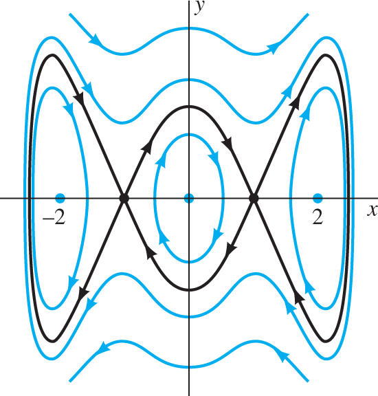
FIGURE 9.4.14.
The phase portrait for Problem 16.
Integrate once (as in Eq. (6)) to derive the energy equation
12y2+V(x)=E,(36)12y2+V(x)=E, where y=dx/dt
y=dx/dt andV(x)=∫x0ϕ(u) du.(37)V(x)=∫x0ϕ(u) du. If the mass is released from rest with initial conditions x(0)=x0, y(0)=0
x(0)=x0, y(0)=0 and periodic oscillations ensue, conclude from Eq. (36) that E=V(x0)E=V(x0) and that the time T required for one complete oscillation isT=4√2∫x00du√V(x0)−V(u).(38)T=42–√∫x00duV(x0)−V(u)−−−−−−−−−−−√. Substitute u=x0cos ϕ
u=x0cos ϕ in (39) to show thatT=2T0π√1−ϵ∫π/20dϕ√1−μsin2ϕ,(40)T=2T0π1−ϵ−−−−√∫π/20dϕ1−μsin2ϕ−−−−−−−−−√, where T0=2π/√k
T0=2π/k−−√ is the linear period,ϵ=βkx20,andμ=−12⋅ϵ1−ϵ.(41)ϵ=βkx20,andμ=−12⋅ϵ1−ϵ. If ϵ=βx20/k
ϵ=βx20/k is sufficiently small that ϵ2ϵ2 is negligible, deduce from Eqs. (41) and (42) thatT≈T0(1+38ϵ)=T0(1+3β8kx20).(43)T≈T0(1+38ϵ)=T0(1+3β8kx20). It follows that
If β>0,
β>0, so the spring is soft, then T>T0,T>T0, and increasing x0x0 increases T, so the larger ovals in Fig. 9.4.4 correspond to smaller frequencies.If β<0,
β<0, so the spring is hard, then T<T0,T<T0, and increasing x0x0 decreases T, so the larger ovals in Fig. 9.4.2 correspond to larger frequencies.
9.4 Application The Rayleigh, van der Pol, and FitzHugh-Nagumo Equations
Here we present a trio of nonlinear differential equations or systems of equations, drawn from the areas of acoustics, electrical engineering, and neuroscience. Each of these models has been fundamental within its field; taken together, they give some indication of the importance of nonlinear equations across a wide variety of applications.
Rayleigh’s Equation
The British mathematical physicist Lord Rayleigh (John William Strutt, 1842–1919) introduced an equation of the form
to model the oscillations of a clarinet reed. With y=x′
whose phase plane portrait is shown in Fig. 9.4.15 (for the case m=k=a=b=1

FIGURE 9.4.15.
Phase plane portrait for the Rayleigh system in (2) with m=k=a=b=1

FIGURE 9.4.16.
The tx-solution curve with initial conditions x(0)=0.01,x′(0)=0
Choose your own parameters m, k, a, and b (perhaps the least four nonzero digits in your student ID number), and use an available ODE plotting utility to plot trajectories and solution curves as in Figs. 9.4.15 and 9.4.16. Change one of your parameters to see how the amplitude and frequency of the resulting periodic oscillations are altered.
Van der Pol’s Equation
Figure 9.4.17 shows a simple RLC circuit in which the usual (passive) resistance R has been replaced with an active element (such as a vacuum tube or semiconductor) across which the voltage drop V is given by a known function f(I) of the current I. Of course, V=f(I)=IR

FIGURE 9.4.17.
A simple circuit with an active element.
In a 1924 study of oscillator circuits in early commercial radios, Balthasar van der Pol (1889–1959) assumed the voltage drop to be given by a nonlinear function of the form f(I)=bI3−aI,
This equation is closely related to Rayleigh’s equation and has phase portraits resembling Fig. 9.4.15. Indeed, differentiation of the second equation in (2) and the resubstitution x′=y
which has the same form as Eq. (4).
If we denote by τ
With p=√a/(3b)
of van der Pol’s equation.
For every nonnegative value of the parameter μ,ode15s. The corresponding x(t) and y(t) solution curves in Figs. 9.4.21 and 9.4.22 reveal surprising behavior of these component functions. Each alternates long intervals of very slow change with periods of abrupt change during very short time intervals that correspond to the “quasi-discontinuities” that are visible in Figs. 9.4.21 and 9.4.22. For instance, Fig. 9.4.23 shows that, between t=1614.28
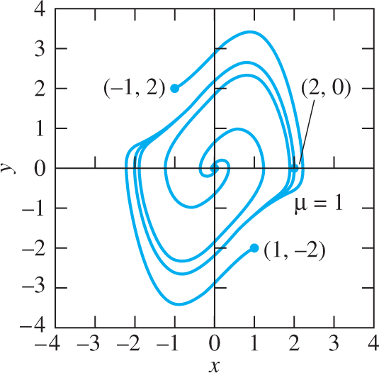
FIGURE 9.4.18.
The phase plane trajectory of a periodic solution of van der Pol’s equation with μ=1,

FIGURE 9.4.19.
x(t) and y(t) solution curves defining the periodic solution of van der Pol’s equation with μ=1

FIGURE 9.4.20.
The phase plane trajectory of the periodic solution of van der Pol’s equation with μ=1000

FIGURE 9.4.21.
Graph of x(t) with μ=1000
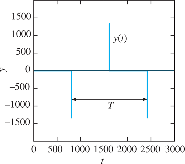
FIGURE 9.4.22.
Graph of y(t) with μ=1000

FIGURE 9.4.23.
The upper spike in the graph of y(t).
You might also plot other trajectories for μ=10, 100
The FitzHugh-Nagumo Equations
Since the early experiments of Luigi Galvani (1737–1798) in which electrical stimulus caused the leg muscles of dead frogs to twitch, the electrical properties of neurons, the cells that form the building blocks of the nervous system, have been intensively studied. One of the most important of those properties is the action potential, an electrical signal that travels from the body of a neuron down along its axon (Fig. 9.4.24). Action potentials are the units of information of the nervous system; when an action potential reaches the end of the axon, chemicals known as neurotransmitters are released from the axon terminals. These neurotransmitters then find receptors in the dendrites of other nerve cells, causing action potentials in those “target” neurons, and thus propagating the “message.” Because of the great speed with which action potentials traverse the neuron, they provide a mechanism by which signals can be rapidly transmitted through the nervous system.
Action potentials are particularly known for their all-or-none character. If the stimulus received by a target neuron is below a certain threshold, then no action potential is generated. If this threshold is exceeded, however, then the neuron will “fire” an action potential, or perhaps (if the stimulus is sufficiently strong) several action potentials in succession. In this way, the nervous system’s method of electrical signaling resembles the binary code used by computers.

FIGURE 9.4.24.
The structure of a typical neuron.
In the early 1950’s A. F. Huxley (1917–2012) and A. L. Hodgkin (1914–1998) published a landmark series of papers in which they modeled the action potential in the giant axon of the squid as an electrical circuit. The focus of this model was the neuron’s membrane potential, that is, the voltage difference between the inside and outside of the nerve cell. In its resting state, a typical neuron has a negative membrane potential, that is, the inside of the cell is at a lower voltage than the surrounding medium. (We now know that this voltage difference is largely due to “ion pumps” in the cell membrane, which maintain a lower concentration of positively charged sodium ions inside the cell than in the surrounding medium. These pumps require energy, and indeed a significant portion of the body’s metabolic energy is devoted to this task.) Potassium ions also play an important role in neuron electrical activity.
During an action potential, the membrane potential exhibits a characteristic pattern of sudden and rapid changes through positive and negative values as the electrical signal traverses the neuron. A central goal of Hodgkin and Huxley’s work was to explain these changes in terms of the sodium and potassium conductances of the neuron membrane. Conductance—the reciprocal of resistance—is a measure of the permeability of the membrane to charged ions. An increase in the sodium conductance, for example, allows sodium ions to flow more freely across the membrane, from areas of high concentration to low. Hodgkin and Huxley proposed that during an action potential, an electrical stimulus (arising from another neuron “upstream,” for example) causes changes in the neuron membrane’s sodium and potassium conductances. This results in a series of flows of charged ions, and thus electrical currents, across the cell membrane.
The researchers applied some of the basic principles of circuit theory to model these currents. The result was a system of four nonlinear differential equations, whose variables are the neuron membrane potential together with three other quantities related to the membrane’s sodium and potassium conductances. Not only did the predictions of this model show remarkable accord with experimental results, they also helped point the way to subsequent discoveries in neurophysiology. The Hodgkin-Huxley model was a triumph both of experimental technique and theoretical analysis, and remains today the starting point for mathematical modeling of action potentials. Together with John Eccles, Hodgkin and Huxley were awarded the 1963 Nobel Prize in Physiology or Medicine for their work.
Analysis of the Hodgkin-Huxley model can be challenging, however, because its phase space is four-dimensional, making features such as solution curves difficult to visualize. For this reason, in 1961 Richard FitzHugh (1922–2007) proposed a two-dimensional simplification of the Hodgkin-Huxley model, which was subsequently analyzed in electrical circuit terms by J. Nagumo and others. Whereas the FitzHugh-Nagumo equations are not intended to capture the physiological properties of the neuron as directly as the original Hodgkin-Huxley equations do, this simplified model is important because it displays much of the qualitative behavior characteristic of neuron electrical activity, while offering the advantage of being considerably easier to study. FitzHugh’s model actually is a generalization of van der Pol’s equation (6). You can show that introduction of the variable y=1μx′+13x3−x
which FitzHugh generalized by adding terms:
Here a and b are constants and I is a function of the time t. Loosely speaking, x(t) behaves in a manner similar to the neuron membrane potential, I(t) is the electrical stimulus applied to the neuron, and y(t) is a composite of the other three variables in the Hodgkin-Huxley model. To simulate neuron electrical activity, we will use FitzHugh’s values a=0.7, b=0.8,
First, with I(t)≡0

FIGURE 9.4.25.
Solutions of the FitzHugh-Nagumo equations (7) with three constant values of the electrical stimulus I(t), using a=0.7,b=0.8,
When the stimulus I(t) is held at the constant value −0.15,
After using your own computer system’s ODE solver to verify these behaviors, you can investigate what happens with other constant nonzero values of the stimulus I(t). Do all such values lead either to oscillatory phase plane solutions or to ones that converge to the same perturbed equilibrium point? Or do certain different values lead to different perturbed equilibrium points? Do all oscillatory solutions correspond to phase plane curves that appear to converge to a single limit cycle?
The FitzHugh-Nagumo system has proven to be a very useful simplification of the Hodgkin-Huxley system, exhibiting a number of characteristics of neuron electrical activity. For a more detailed discussion see the classic work of L. Edelstein-Keshet, Mathematical Models in Biology (Society for Industrial and Applied Mathematics, 2005).