Search in book...
Toggle Font Controls
Create new playlist

Name your new playlist

Playlist description (optional)
Sign In

Email address

Password

Forgot Password?

or

Continue with Facebook

Continue with Google
Sign Up

Full Name

Email address

Confirm Email Address

Password

or

Continue with Facebook

Continue with Google

5.4 Mechanical Vibrations

The motion of a mass attached to a spring serves as a relatively simple example of the vibrations that occur in more complex mechanical systems. For many such systems, the analysis of these vibrations is a problem in the solution of linear differential equations with constant coefficients.

We consider a body of mass m attached to one end of an ordinary spring that resists compression as well as stretching; the other end of the spring is attached to a fixed wall, as shown in Fig. 5.4.1. Assume that the body rests on a frictionless horizontal plane, so that it can move only back and forth as the spring compresses and stretches. Denote by x the distance of the body from its equilibrium position—its position when the spring is unstretched. We take x>0 $x > 0$ when the spring is stretched, and thus x<0 $x < 0$ when it is compressed.

FIGURE 5.4.1.

A mass–spring–dashpot system.

According to Hooke’s law, the restorative force FS $F_{S}$ that the spring exerts on the mass is proportional to the distance x that the spring has been stretched or compressed. Because this is the same as the displacement x of the mass m from its equilibrium position, it follows that

F S = - k x .

$F_{S} = - k x .$ (1)

The positive constant of proportionality k is called the spring constant. Note that FS $F_{S}$ and x have opposite signs: FS<0 $F_{S} < 0$ when x>0, FS>0 $x > 0, F_{S} > 0$ when x<0 $x < 0$ .

Figure 5.4.1 shows the mass attached to a dashpot—a device, like a shock absorber, that provides a force directed opposite to the instantaneous direction of motion of the mass m. We assume the dashpot is so designed that this force FR $F_{R}$ is proportional to the velocity v=dx/dt $v = d x / d t$ of the mass; that is,

F R = - c v = - c d x d t .

$F_{R} = - c v = - c \frac{d x}{d t} .$ (2)

The positive constant c is the damping constant of the dashpot. More generally, we may regard Eq. (2) as specifying frictional forces in our system (including air resistance to the motion of m).

If, in addition to the forces FS $F_{S}$ and FR, $F_{R},$ the mass is subjected to a given external force FE=F(t), $F_{E} = F (t),$ then the total force acting on the mass is F=FS+FR+FE. $F = F_{S} + F_{R} + F_{E} .$ Using Newton’s law

F = m a = m d 2 x d t 2 = m x'',

$F = m a = m \frac{d^{2} x}{d t^{2}} = m x ″,$

we obtain the second-order linear differential equation

m x'' + c x' + k x = F (t)

$m x ″ + c x ′ + k x = F (t)$ (3)

that governs the motion of the mass.

If there is no dashpot (and we ignore all frictional forces), then we set c=0 $c = 0$ in Eq. (3) and call the motion undamped; it is damped motion if c>0. $c > 0 .$ If there is no external force, we replace F(t) with 0 in Eq. (3). We refer to the motion as free in this case and forced in the case F(t)≠0. $F (t) \neq 0 .$ Thus the homogeneous equation

m x'' + c x' + k x = 0

$m x ″ + c x ′ + k x = 0$ (4)

describes free motion of a mass on a spring with dashpot but with no external forces applied. We will defer discussion of forced motion until Section 5.6.

For an alternative example, we might attach the mass to the lower end of a spring that is suspended vertically from a fixed support, as in Fig. 5.4.2. In this case the weight W=mg $W = m g$ of the mass would stretch the spring a distance s0 $s_{0}$ determined by Eq. (1) with FS=−W $F_{S} = - W$ and x=s0. $x = s_{0} .$ That is, mg=ks0, $m g = k s_{0},$ so that s0=mg/k. $s_{0} = m g / k .$ This gives the static equilibrium position of the mass. If y denotes the displacement of the mass in motion, measured downward from its static equilibrium position, then we ask you to show in Problem 9 that y satisfies Eq. (3); specifically, that

m y'' + c y' + k y = F (t)

$m y ″ + c y ′ + k y = F (t)$ (5)

FIGURE 5.4.2.

A mass suspended vertically from a spring.

if we include damping and external forces (meaning those other than gravity).

The Simple Pendulum

The importance of the differential equation that appears in Eqs. (3) and (5) stems from the fact that it describes the motion of many other simple mechanical systems. For example, a simple pendulum consists of a mass m swinging back and forth on the end of a string (or better, a massless rod) of length L, as shown in Fig. 5.4.3. We may specify the position of the mass at time t by giving the counterclockwise angle θ=θ(t) $θ = θ (t)$ that the string or rod makes with the vertical at time t. To analyze the motion of the mass m, we will apply the law of the conservation of mechanical energy, according to which the sum of the kinetic energy and the potential energy of m remains constant.

The distance along the circular arc from 0 to m is s=Lθ, $s = L θ,$ so the velocity of the mass is v=ds/dt=L(dθ/dt), $v = d s / d t = L (d θ / d t),$ and therefore its kinetic energy is

T = 1 2 m v 2 = 1 2 m (d s d t) 2 = 1 2 m L 2 (d θ d t) 2 .

$T = \frac{1}{2} m v^{2} = \frac{1}{2} m {(\frac{d s}{d t})}^{2} = \frac{1}{2} m L^{2} {(\frac{d θ}{d t})}^{2} .$

We next choose as reference point the lowest point O reached by the mass (see Fig. 5.4.3). Then its potential energy V is the product of its weight mg and its vertical height h=L(1−cos θ) $h = L (1 - \cos θ)$ above O, so

V = m g L (1 - cos θ) .

$V = m g L (1 - \cos θ) .$

The fact that the sum of T and V is a constant C therefore gives

1 2 m L 2 (d θ d t) 2 + m g L (1 - cos θ) = C .

$\frac{1}{2} m L^{2} {(\frac{d θ}{d t})}^{2} + m g L (1 - \cos θ) = C .$

We differentiate both sides of this identity with respect to t to obtain

m L 2 (d θ d t) (d 2 θ d t 2) + m g L (sin θ) d θ d t = 0,

$m L^{2} (\frac{d θ}{d t}) (\frac{d^{2} θ}{d t^{2}}) + m g L (\sin θ) \frac{d θ}{d t} = 0,$

d 2 θ d t 2 + g L sin θ = 0

$\frac{d^{2} θ}{d t^{2}} + \frac{g}{L} \sin θ = 0$ (6)

after removal of the common factor mL2(dθ/dt). $m L^{2} (d θ / d t) .$ This differential equation can be derived in a seemingly more elementary manner using the familiar second law F=ma $F = m a$ of Newton (applied to tangential components of the acceleration of the mass and the force acting on it). However, derivations of differential equations based on conservation of energy are often seen in more complex situations where Newton’s law is not so directly applicable, and it may be instructive to see the energy method in a simpler application like the pendulum.

Now recall that if θ $θ$ is small, then sin θ≈θ $\sin θ \approx θ$ (this approximation obtained by retaining just the first term in the Taylor series for sin θ $\sin θ$ ). In fact, sin θ $\sin θ$ and θ $θ$ agree to two decimal places when |θ| $| θ |$ is at most π/12 $π / 12$ (that is, 15° $15 °$ ). In a typical pendulum clock, for example, θ $θ$ would never exceed 15° $15 °$ . It therefore seems reasonable to simplify our mathematical model of the simple pendulum by replacing sin θ $\sin θ$ with θ $θ$ in Eq. (6). If we also insert a term cθ' $c θ ′$ to account for the frictional resistance of the surrounding medium, the result is an equation in the form of Eq. (4):

θ'' + c θ' + k θ = 0

$θ ″ + c θ ′ + k θ = 0$ (7)

where k=g/L. $k = g / L .$ Note that this equation is independent of the mass m on the end of the rod. We might, however, expect the effects of the discrepancy between θ $θ$ and sin θ $\sin θ$ to accumulate over a period of time, so that Eq. (7) will probably not describe accurately the actual motion of the pendulum over a long period of time.

In the remainder of this section, we first analyze free undamped motion and then free damped motion.

Free Undamped Motion

If we have only a mass on a spring, with neither damping nor external force, then Eq. (3) takes the simpler form

m x'' + k x = 0.

$m x ″ + k x = 0.$ (8)

It is convenient to define

ω 0 = k m - - - \sqrt

$ω_{0} = \sqrt{\frac{k}{m}}$ (9)

and rewrite Eq. (8) as

x'' + ω 20 x = 0.

$x ″ + ω_{0}^{2} x = 0.$ (8′)

The general solution of Eq. (8′) is

x (t) = A cos ω 0 t + B sin ω 0 t .

$x (t) = A \cos ω_{0} t + B \sin ω_{0} t .$ (10)

To analyze the motion described by this solution, we choose constants C and α $α$ so that

C = A 2 + B 2 - - - - - - - \sqrt, cos α = A C, and sin α = B C,

$C = \sqrt{A^{2} + B^{2}}, \cos α = \frac{A}{C}, and \sin α = \frac{B}{C},$ (11)

as indicated in Fig. 5.4.4. Note that, although tanα=B/A, $\tan α = B / A,$ the angle α $α$ is not given by the principal branch of the inverse tangent function (which gives values only in the interval −π/2<x<π/2 $- π / 2 < x < π / 2$ ). Instead, α $α$ is the angle between 0 and 2π $2 π$ whose cosine and sine have the signs given in (11), where either A or B or both may be negative. Thus

α = ⎧ ⎩ ⎨ ⎪ ⎪ tan - 1 (B / A) π + tan - 1 (B / A) 2 π + tan - 1 (B / A) if A > 0, B > 0 (first quadrant), if A < 0 (second or third quadrant), if A > 0, B < 0 (fourth quadrant),

$α = {\begin{array}{l} \tan^{- 1} (B / A) & if A > 0, B > 0 (first quadrant), \\ π + \tan^{- 1} (B / A) & if A < 0 (second or third quadrant), \\ 2 π + \tan^{- 1} (B / A) & if A > 0, B < 0 (fourth quadrant), \end{array}$

where tan−1(B/A) $\tan^{- 1} (B / A)$ is the angle in (−π/2,π/2) $(- π / 2, π / 2)$ given by a calculator or computer.

In any event, from (10) and (11) we get

x (t) = C (A C cos ω 0 t + B C sin ω 0 t) = C (cos α cos ω 0 t + sin α sin ω 0 t) .

$x (t) = C (\frac{A}{C} \cos ω_{0} t + \frac{B}{C} \sin ω_{0} t) = C (\cos α \cos ω_{0} t + \sin α \sin ω_{0} t) .$

With the aid of the cosine addition formula, we find that

x (t) = C cos (ω 0 t - α) .

$x (t) = C \cos (ω_{0} t - α) .$ (12)

Thus the mass oscillates to and fro about its equilibrium position with

Amplitude C,
Circular frequency ω0 $ω_{0}$ , and
Phase angle α $α$ .

Such motion is called simple harmonic motion.

If time t is measured in seconds, the circular frequency ω0 $ω_{0}$ has dimensions of radians per second (rad/s). The period of the motion is the time required for the system to complete one full oscillation, so is given by

T = 2 π ω 0

$T = \frac{2 π}{ω_{0}}$ (13)

seconds; its frequency is

v = 1 T = ω 0 2 π

$v = \frac{1}{T} = \frac{ω_{0}}{2 π}$ (14)

in hertz (Hz), which measures the number of complete cycles per second. Note that frequency is measured in cycles per second, whereas circular frequency has the dimensions of radians per second.

A typical graph of a simple harmonic position function

x (t) = C cos (ω 0 t - α) = C cos (ω 0 (t - α ω 0)) = C cos (ω 0 (t - δ))

$x (t) = C \cos (ω_{0} t - α) = C \cos (ω_{0} (t - \frac{α}{ω_{0}})) = C \cos (ω_{0} (t - δ))$

is shown in Fig. 5.4.5, where the geometric significance of the amplitude C, the period T, and the time lag

δ = α ω 0

$δ = \frac{α}{ω_{0}}$

are indicated.

If the initial position x(0)=x0 $x (0) = x_{0}$ and initial velocity x'(0)=v0 $x ′ (0) = v_{0}$ of the mass are given, we first determine the values of the coefficients A and B in Eq. (10), then find the amplitude C and phase angle α $α$ by carrying out the transformation of x(t) to the form in Eq. (12), as indicated previously.

Example 1

Undamped mass-spring system A body with mass m=12 $m = \frac{1}{2}$ kilogram (kg) is attached to the end of a spring that is stretched 2 meters (m) by a force of 100 newtons (N). It is set in motion with initial position x0=1 $x_{0} = 1$ (m) and initial velocity v0=−5 $v_{0} = - 5$ (m/s). (Note that these initial conditions indicate that the body is displaced to the right and is moving to the left at time t=0 $t = 0$ .) Find the position function of the body as well as the amplitude, frequency, period of oscillation, and time lag of its motion.

Solution

The spring constant is k=(100N)/(2m)=50 $k = (100 N) / (2 m) = 50$ (N/m), so Eq. (8) yields 12x''+50x=0; $\frac{1}{2} x ″ + 50 x = 0;$ that is,

x'' + 100 x = 0.

$x ″ + 100 x = 0.$

Consequently, the circular frequency of the resulting simple harmonic motion of the body will be ω0=100−−−√=10 $ω_{0} = \sqrt{100} = 10$ (rad/s). Hence it will oscillate with period

T = 2 π ω 0 = 2 π 10 \approx 0.6283 s

$T = \frac{2 π}{ω_{0}} = \frac{2 π}{10} \approx 0.6283 s$

and with frequency

v = 1 T = ω 0 2 π = 10 2 π \approx 1.5915 Hz .

$v = \frac{1}{T} = \frac{ω_{0}}{2 π} = \frac{10}{2 π} \approx 1.5915 Hz .$

We now impose the initial conditions x(0)=1 $x (0) = 1$ and x'(0)=−5 $x ′ (0) = - 5$ on the position function

x (t) = A cos 10 t + B sin 10 t with x' (t) = - 10 A sin 10 t + 10 B cos 10 t .

$x (t) = A \cos 10 t + B \sin 10 t with x ′ (t) = - 10 A \sin 10 t + 10 B \cos 10 t .$

It follows readily that A=1 $A = 1$ and B=−12, $B = - \frac{1}{2},$ so the position function of the body is

x (t) = cos 10 t - 1 2 sin 10 t .

$x (t) = \cos 10 t - \frac{1}{2} \sin 10 t .$

Hence its amplitude of motion is

C = (1) 2 + (- 1 2) 2 - - - - - - - - - - \sqrt = 1 2 5 - \sqrt m .

$C = \sqrt{{(1)}^{2} + {(- \frac{1}{2})}^{2}} = \frac{1}{2} \sqrt{5} m .$

To find the time lag, we write

x (t) = 5 - \sqrt 2 (2 5 - \sqrt cos 10 t - 1 5 - \sqrt sin 10 t) = 5 - \sqrt 2 cos (10 t - α),

$x (t) = \frac{\sqrt{5}}{2} (\frac{2}{\sqrt{5}} \cos 10 t - \frac{1}{\sqrt{5}} \sin 10 t) = \frac{\sqrt{5}}{2} \cos (10 t - α),$

where the phase angle α $α$ satisfies

cos α = 2 5 - \sqrt > 0 and sin α = - 1 5 - \sqrt < 0.

$\cos α = \frac{2}{\sqrt{5}} > 0 and \sin α = - \frac{1}{\sqrt{5}} < 0.$

Hence α $α$ is the fourth-quadrant angle

α = 2 π + tan - 1 (- 1 / 5 - \sqrt 2 / 5 - \sqrt) = 2 π - tan - 1 (1 2) \approx 5.8195,

$α = 2 π + \tan^{- 1} (\frac{- 1 / \sqrt{5}}{2 / \sqrt{5}}) = 2 π - \tan^{- 1} (\frac{1}{2}) \approx 5.8195,$

and the time lag of the motion is

δ = α ω 0 \approx 0.5820 s .

$δ = \frac{α}{ω_{0}} \approx 0.5820 s .$

With the amplitude and approximate phase angle shown explicitly, the position function of the body takes the form

x (t) \approx 1 2 5 - \sqrt cos (10 t - 5.8195),

$x (t) \approx \frac{1}{2} \sqrt{5} \cos (10 t - 5.8195),$

and its graph is shown in Fig. 5.4.6.

FIGURE 5.4.6.

Graph of the position function x(t)≈C cos(ω0t−α) $x (t) \approx C \cos (ω_{0} t - α)$ in Example 1, with amplitude C≈1.118, $C \approx 1.118,$ period T≈0.628, $T \approx 0.628,$ and time δ≈0.582. $δ \approx 0.582.$

Free Damped Motion

With damping but no external force, the differential equation we have been studying takes the form mx''+cx'+kx=0; $m x ″ + c x ′ + k x = 0;$ alternatively,

x'' + 2 p x' + ω 20 x = 0,

$x ″ + 2 p x ′ + ω_{0}^{2} x = 0,$ (15)

where ω0=k/m−−−−√ $ω_{0} = \sqrt{k / m}$ is the corresponding undamped circular frequency and

p = c 2 m > 0.

$p = \frac{c}{2 m} > 0.$ (16)

The characteristic equation r2+2pr+ω20=0 $r^{2} + 2 p r + ω_{0}^{2} = 0$ of Eq. (15) has roots

r 1, r 2 = - p \pm (p 2 - ω 20) 1/2

$r_{1}, r_{2} = - p \pm {(p^{2} - ω_{0}^{2})}^{1/2}$ (17)

that depend on the sign of

p 2 - ω 20 = c 2 4 m 2 - k m = c 2 - 4 k m 4 m 2 .

$p^{2} - ω_{0}^{2} = \frac{c^{2}}{4 m^{2}} - \frac{k}{m} = \frac{c^{2} - 4 k m}{4 m^{2}} .$ (18)

The critical damping ccr $c_{cr}$ is given by ccr=4km−−−−√, $c_{cr} = \sqrt{4 k m},$ and we distinguish three cases, according as c>ccr, c=ccr, $c > c_{cr}, c = c_{cr},$ or c<ccr $c < c_{cr}$ .

Overdamped Case: c>ccr (c2>4k m). $c > c_{cr} (c^{2} > 4 k m) .$ Because c is relatively large in this case, we are dealing with a strong resistance in comparison with a relatively weak spring or a small mass. Then (17) gives distinct real roots r1 $r_{1}$ and r2, $r_{2},$ both of which are negative. The position function has the form

x (t) = c 1 e r 1 t + c 2 e r 2 t .

$x (t) = c_{1} e^{r_{1} t} + c_{2} e^{r_{2} t} .$ (19)

It is easy to see that x(t)→0 $x (t) \to 0$ as t→+∞ $t \to + \infty$ and that the body settles to its equilibrium position without any oscillations (Problem 29). Figure 5.4.7 shows some typical graphs of the position function for the overdamped case; we chose x0 $x_{0}$ a fixed positive number and illustrated the effects of changing the initial velocity v0. $v_{0} .$ In every case the would-be oscillations are damped out.

FIGURE 5.4.7.

Overdamped motion: x(t)=c1er1t+c2er2t $x (t) = c_{1} e^{r_{1} t} + c_{2} e^{r_{2} t}$ with r1<0 $r_{1} < 0$ and r2<0. $r_{2} < 0.$ Solution curves are graphed with the same initial position x0 $x_{0}$ and different initial velocities.

Critically Damped Case: c=ccr (c2=4k m). $c = c_{cr} (c^{2} = 4 k m) .$ In this case, (17) gives equal roots r1=r2=−p $r_{1} = r_{2} = - p$ of the characteristic equation, so the general solution is

x (t) = e - p t (c 1 + c 2 t) .

$x (t) = e^{- p t} (c_{1} + c_{2} t) .$ (20)

Because e−pt>0 $e^{- p t} > 0$ and c1+c2t $c_{1} + c_{2} t$ has at most one positive zero, the body passes through its equilibrium position at most once, and it is clear that x(t)→0 $x (t) \to 0$ as t→+∞. $t \to + \infty .$ Some graphs of the motion in the critically damped case appear in Fig. 5.4.8, and they resemble those of the overdamped case (Fig. 5.4.7). In the critically damped case, the resistance of the dashpot is just large enough to damp out any oscillations, but even a slight reduction in resistance will bring us to the remaining case, the one that shows the most dramatic behavior.

FIGURE 5.4.8.

Critically damped motion: x(t)=(c1+c2t)e−pt $x (t) = (c_{1} + c_{2} t) e^{- p t}$ with p>0. $p > 0.$ Solution curves are graphed with the same initial position x0 $x_{0}$ and different initial velocities.

Underdamped Case: c<ccr (c2<4k m). $c < c_{cr} (c^{2} < 4 k m) .$ The characteristic equation now has two complex conjugate roots −p±iω20−p2−−−−−−√, $- p \pm i \sqrt{ω_{0}^{2} - p^{2}},$ and the general solution is

x (t) = e - p t (A cos ω 1 t + B sin ω 1 t),

$x (t) = e^{- p t} (A \cos ω_{1} t + B \sin ω_{1} t),$ (21)

where

ω 1 = ω 20 - p 2 - - - - - - \sqrt = 4 k m - c 2 - - - - - - - - \sqrt 2 m .

$ω_{1} = \sqrt{ω_{0}^{2} - p^{2}} = \frac{\sqrt{4 k m - c^{2}}}{2 m} .$ (22)

Using the cosine addition formula as in the derivation of Eq. (12), we may rewrite Eq. (20) as

x (t) = C e - p t (A C cos ω 1 t + B C sin ω 1 t),

$x (t) = C e^{- p t} (\frac{A}{C} \cos ω_{1} t + \frac{B}{C} \sin ω_{1} t),$

x (t) = C e - p t cos (ω 1 t - α)

$x (t) = C e^{- p t} \cos (ω_{1} t - α)$ (23)

where

C = A 2 + B 2 - - - - - - - \sqrt, cos α = A C, and sin α = B C .

$C = \sqrt{A^{2} + B^{2}}, \cos α = \frac{A}{C}, and \sin α = \frac{B}{C} .$

The solution in (21) represents exponentially damped oscillations of the body around its equilibrium position. The graph of x(t) lies between the “amplitude envelope” curves x=−Ce−pt $x = - C e^{- p t}$ and x=Ce−pt $x = C e^{- p t}$ and touches them when ω1t−α $ω_{1} t - α$ is an integral multiple of π. $π .$ The motion is not actually periodic, but it is nevertheless useful to call ω1 $ω_{1}$ its circular frequency (more properly, its pseudofrequency), T1=2π/ω1 $T_{1} = 2 π / ω_{1}$ its pseudoperiod of oscillation, and Ce−pt $C e^{- p t}$ its time-varying amplitude. Most of these quantities are shown in the typical graph of underdamped motion in Fig. 5.4.9. Note from Eq. (22) that in this case ω1 $ω_{1}$ is less than the undamped circular frequency ω0, $ω_{0},$ so T1 $T_{1}$ is larger than the period T of oscillation of the same mass without damping on the same spring. Thus the action of the dashpot has at least two effects:

FIGURE 5.4.9.

Underdamped oscillations: x(t)=Ce−ptcos(ω1t−α) $x (t) = C e^{- p t} \cos (ω_{1} t - α)$ .

It exponentially damps the oscillations, in accord with the time-varying amplitude.
It slows the motion; that is, the dashpot decreases the frequency of the motion.

As the following example illustrates, damping typically also delays the motion further—that is, increases the time lag—as compared with undamped motion with the same initial conditions.

Example 2

Damped system The mass and spring of Example 1 are now attached also to a dashpot that provides 1 N of resistance for each meter per second of velocity. The mass is set in motion with the same initial position x(0)=1 $x (0) = 1$ and initial velocity x'(0)=−5 $x ′ (0) = - 5$ as in Example 1. Now find the position function of the mass, its new frequency and pseudoperiod of motion, its new time lag, and the times of its first four passages through the initial position x=0 $x = 0$ .

Solution

Rather than memorizing the various formulas given in the preceding discussion, it is better practice in a particular case to set up the differential equation and then solve it directly. Recall that m=12 $m = \frac{1}{2}$ and k=50; $k = 50;$ we are now given c=1 $c = 1$ in mks units. Hence Eq. (4) is 12x''+x'+50x=0; $\frac{1}{2} x ″ + x ′ + 50 x = 0;$ that is,

x'' + 2 x' + 100 x = 0.

$x ″ + 2 x ′ + 100 x = 0.$

The characteristic equation r2+2r+100=(r+1)2+99=0 $r^{2} + 2 r + 100 = {(r + 1)}^{2} + 99 = 0$ has roots r1, r2=−1±99−−√i, $r_{1}, r_{2} = - 1 \pm \sqrt{99} i,$ so the general solution is

x (t) = e - t (A cos 99 - - \sqrt t + B sin 99 - - \sqrt t) .

$x (t) = e^{- t} (A \cos \sqrt{99} t + B \sin \sqrt{99} t) .$ (24)

Consequently, the new circular (pseudo)frequency is ω1=99−−√≈9.9499 $ω_{1} = \sqrt{99} \approx 9.9499$ (as compared with ω0=10 $ω_{0} = 10$ in Example 1). The new (pseudo)period and frequency are

T 1 = 2 π ω 1 = 2 π 99 - - \sqrt \approx 0.6315 s

$T_{1} = \frac{2 π}{ω_{1}} = \frac{2 π}{\sqrt{99}} \approx 0.6315 s$

and

v 1 = 1 T 1 = ω 1 2 π = 99 - - \sqrt 2 π \approx 1.5836 Hz

$v_{1} = \frac{1}{T_{1}} = \frac{ω_{1}}{2 π} = \frac{\sqrt{99}}{2 π} \approx 1.5836 Hz$

(as compared with T≈0.6283<T1 $T \approx 0.6283 < T_{1}$ and ν≈1.5915>ν1 $ν \approx 1.5915 > ν_{1}$ in Example 1).

We now impose the initial conditions x(0)=1 $x (0) = 1$ and x'(0)=−5 $x ′ (0) = - 5$ on the position function in (23) and the resulting velocity function

x' (t) = - e - t (A cos 99 - - \sqrt t + B sin 99 - - \sqrt t) + 99 - - \sqrt e - t (- A sin 99 - - \sqrt t + B cos 99 - - \sqrt t) .

$x^{′} (t) = - e^{- t} (A \cos \sqrt{99} t + B \sin \sqrt{99} t) + \sqrt{99} e^{- t} (- A \sin \sqrt{99} t + B \cos \sqrt{99} t) .$

It follows that

x (0) = A = 1 and x' (0) = - A + B 99 - - \sqrt = - 5,

$x (0) = A = 1 and x^{′} (0) = - A + B \sqrt{99} = - 5,$

whence we find that A=1 $A = 1$ and B=−4/99−−√. $B = - 4 / \sqrt{99} .$ Thus the new position function of the body is

x (t) = e - t (cos 99 - - \sqrt t - 4 99 - - \sqrt sin 99 - - \sqrt t) .

$x (t) = e^{- t} (\cos \sqrt{99} t - \frac{4}{\sqrt{99}} \sin \sqrt{99} t) .$

Hence its time-varying amplitude of motion is

C 1 e - t = (1) 2 + (- 4 99 - - \sqrt) 2 - - - - - - - - - - - - - - - \sqrt e - t = 115 99 - - - - \sqrt e - t .

$C_{1} e^{- t} = \sqrt{{(1)}^{2} + {(- \frac{4}{\sqrt{99}})}^{2}} e^{- t} = \sqrt{\frac{115}{99}} e^{- t} .$

We therefore write

x (t) = = 115 - - - \sqrt 99 - - \sqrt e - t (99 - - \sqrt 115 - - - \sqrt cos 99 - - \sqrt t - 4 115 \sqrt sin 99 - - \sqrt t) 115 - - - \sqrt 99 - - \sqrt e - t cos (99 - - \sqrt t - α 1),

$\begin{aligned} x (t) & = & \frac{\sqrt{115}}{\sqrt{99}} e^{- t} (\frac{\sqrt{99}}{\sqrt{115}} \cos \sqrt{99} t - \frac{4}{\sqrt{115}} \sin \sqrt{99} t) \\ = & \frac{\sqrt{115}}{\sqrt{99}} e^{- t} \cos (\sqrt{99} t - α_{1}), \end{aligned}$

where the phase angle α1 $α_{1}$ satisfies

cos α 1 = 99 - - \sqrt 115 - - - \sqrt > 0 and sin α 1 = - 4 115 - - - \sqrt < 0.

$\cos α_{1} = \frac{\sqrt{99}}{\sqrt{115}} > 0 and \sin α_{1} = - \frac{4}{\sqrt{115}} < 0.$

Hence α1 $α_{1}$ is the fourth-quadrant angle

α 1 = 2 π + tan - 1 (- 4 / 115 - - - \sqrt 99 - - \sqrt / 115 - - - \sqrt) = 2 π - tan - 1 (4 99 - - \sqrt) \approx 5.9009,

$α_{1} = 2 π + \tan^{- 1} (\frac{- 4 / \sqrt{115}}{\sqrt{99} / \sqrt{115}}) = 2 π - \tan^{- 1} (\frac{4}{\sqrt{99}}) \approx 5.9009,$

and the time lag of the motion is

δ 1 = α 1 ω 1 \approx 0.5931 s

$δ_{1} = \frac{α_{1}}{ω_{1}} \approx 0.5931 s$

(as compared with δ≈0.5820<δ1 $δ \approx 0.5820 < δ_{1}$ in Example 1). With the time-varying amplitude and approximate phase angle shown explicitly, the position function of the mass takes the form

x (t) \approx 115 99 - - - - \sqrt e - t cos (99 - - \sqrt t - 5.9009),

$x (t) \approx \sqrt{\frac{115}{99}} e^{- t} \cos (\sqrt{99} t - 5.9009),$ (25)

and its graph is the damped exponential that is shown in Fig. 5.4.10 (in comparison with the undamped oscillations of Example 1).

From (24) we see that the mass passes through its equilibrium position x=0 $x = 0$ when cos(ω1t−α1)=0, $\cos (ω_{1} t - α_{1}) = 0,$ and thus when

ω 1 t - α 1 = - 3 π 2, - π 2, π 2, 3 π 2, \dots;

$ω_{1} t - α_{1} = - \frac{3 π}{2}, - \frac{π}{2}, \frac{π}{2}, \frac{3 π}{2}, \dots;$

that is, when

t = δ 1 - 3 π 2 ω 1, δ 1 - π 2 ω 1, δ 1 + π 2 ω 1, δ 1 + 3 π 2 ω 1, \dots .

$t = δ_{1} - \frac{3 π}{2 ω_{1}}, δ_{1} - \frac{π}{2 ω_{1}}, δ_{1} + \frac{π}{2 ω_{1}}, δ_{1} + \frac{3 π}{2 ω_{1}}, \dots .$

We see similarly that the undamped mass of Example 1 passes through equilibrium when

t = δ 0 - 3 π 2 ω 0, δ 0 - π 2 ω 0, δ 0 + π 2 ω 0, δ 0 + 3 π 2 ω 0, \dots .

$t = δ_{0} - \frac{3 π}{2 ω_{0}}, δ_{0} - \frac{π}{2 ω_{0}}, δ_{0} + \frac{π}{2 ω_{0}}, δ_{0} + \frac{3 π}{2 ω_{0}}, \dots .$

The following table compares the first four values t1,t2,t3,t4 $t_{1}, t_{2}, t_{3}, t_{4}$ we calculate for the undamped and damped cases, respectively.

`n`	1	2	3	4
tn $t_{n}$ (undamped)	0.1107	0.4249	0.7390	1.0532
tn $t_{n}$ (damped)	0.1195	0.4352	0.7509	1.0667

Accordingly, in Fig. 5.4.11 (where only the first three equilibrium passages are shown) we see the damped oscillations lagging slightly behind the undamped ones.

FIGURE 5.4.10.

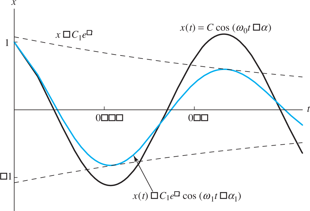
Graphs of the position function x(t)=C1e−tcos(ω1t−α1) $x (t) = C_{1} e^{- t} \cos (ω_{1} t - α_{1})$ of Example 2 (damped oscillations), the position function x(t)=C cos(ω0t−α) $x (t) = C \cos (ω_{0} t - α)$ of Example 1 (undamped oscillations), and the envelope curves x(t)=±C1e−t. $x (t) = \pm C_{1} e^{- t} .$

FIGURE 5.4.11.

Graphs on the interval 0≤t≤0.8 $0 \leq t \leq 0.8$ illustrating the additional delay associated with damping.

5.4 Problems

Determine the period and frequency of the simple harmonic motion of a 4-kg mass on the end of a spring with spring constant 16 N/m.
Determine the period and frequency of the simple harmonic motion of a body of mass 0.75 kg $0.75 kg$ on the end of a spring with spring constant 48 N/m.
A mass of 3 kg is attached to the end of a spring that is stretched 20 cm by a force of 15 N. It is set in motion with initial position x0=0 $x_{0} = 0$ and initial velocity v0=−10 m/s. $v_{0} = - 10 m/s .$ Find the amplitude, period, and frequency of the resulting motion.
A body with mass 250 g is attached to the end of a spring that is stretched 25 cm by a force of 9 N. At time t=0 $t = 0$ the body is pulled 1 m to the right, stretching the spring, and set in motion with an initial velocity of 5 m/s $5 m/s$ to the left. (a) Find x(t) in the form Ccos(ω0t−α). $C \cos (ω_{0} t - α) .$ (b) Find the amplitude and period of motion of the body.

Simple Pendulum

In Problems 5 through 8, assume that the differential equation of a simple pendulum of length L is Lθ''+gθ=0, $L θ ″ + g θ = 0,$ where g=GM/R2 $g = G M / R^{2}$ is the gravitational acceleration at the location of the pendulum (at distance R from the center of the earth; M denotes the mass of the earth).

Two pendulums are of lengths L1 $L_{1}$ and L2 $L_{2}$ and—when located at the respective distances R1 $R_{1}$ and R2 $R_{2}$ from the center of the earth—have periods p1 $p_{1}$ and p2. $p_{2} .$ Show that

$p 1 p 2 = R 1 L 1 - - \sqrt R 2 L 2 - - \sqrt .$ $\frac{p_{1}}{p_{2}} = \frac{R_{1} \sqrt{L_{1}}}{R_{2} \sqrt{L_{2}}} .$
A certain pendulum keeps perfect time in Paris, where the radius of the earth is R=3956 $R = 3956$ (mi). But this clock loses 2 min 40 s per day at a location on the equator. Use the result of Problem 5 to find the amount of the equatorial bulge of the earth.
A pendulum of length 100.10 in., located at a point at sea level where the radius of the earth is R=3960 $R = 3960$ (mi), has the same period as does a pendulum of length 100.00 in. atop a nearby mountain. Use the result of Problem 5 to find the height of the mountain.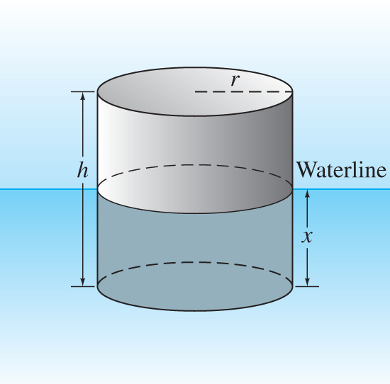

FIGURE 5.4.12.

The buoy of Problem 10.
Most grandfather clocks have pendulums with adjustable lengths. One such clock loses 10 min per day when the length of its pendulum is 30 in. With what length pendulum will this clock keep perfect time?
Derive Eq. (5) describing the motion of a mass attached to the bottom of a vertically suspended spring. (Suggestion: First denote by x(t) the displacement of the mass below the unstretched position of the spring; set up the differential equation for x. Then substitute y=x−s0 $y = x - s_{0}$ in this differential equation.)
Floating buoy Consider a floating cylindrical buoy with radius r, height h, and uniform density ρ≦0.5 $ρ ≦ 0.5$ (recall that the density of water is 1 g/cm3 $1 {g/cm}^{3}$ ). The buoy is initially suspended at rest with its bottom at the top surface of the water and is released at time t=0. $t = 0 .$ Thereafter it is acted on by two forces: a downward gravitational force equal to its weight $m g = ρ π r^{2} h g$ and (by Archimedes’ principle of buoyancy) an upward force equal to the weight $π r^{2} x g$ of water displaced, where $x = x (t)$ is the depth of the bottom of the buoy beneath the surface at time t (Fig. 5.4.12). Assume that friction is negligible. Conclude that the buoy undergoes simple harmonic motion around its equilibrium position $x_{e} = ρ h$ with period $p = 2 π \sqrt{ρ h / g} .$ Compute p and the amplitude of the motion if $ρ = 0.5 {g/cm}^{3}, h = 200$ cm, and $g = 980$ c ${m/s}^{2} .$
Floating buoy A cylindrical buoy weighing 100 lb (thus of mass $m = 3.125$ slugs in ft-lb-s (fps)units) floats in water with its axis vertical (as in Problem 10). When depressed slightly and released, it oscillates up and down four times every 10 s. Find the radius of the buoy.
Hole through the earth Assume that the earth is a solid sphere of uniform density, with mass M and radius $R = 3960$ (mi). For a particle of mass m within the earth at distance r from the center of the earth, the gravitational force attracting m toward the center is $F_{r} = - {G M}_{r} m / r^{2},$ where $M_{r}$ is the mass of the part of the earth within a sphere of radius r (Fig. 5.4.13). (a) Show that $F_{r} = - G M m r / R^{3} .$

FIGURE 5.4.13.

A mass m falling down a hole through the center of the earth (Problem 12).

(b) Now suppose that a small hole is drilled straight through the center of the earth, thus connecting two antipodal points on its surface. Let a particle of mass m be dropped at time $t = 0$ into this hole with initial speed zero, and let r(t) be its distance from the center of the earth at time t, where we take $r < 0$ when the mass is “below” the center of the earth. Conclude from Newton’s second law and part (a) that $r ″ (t) = - k^{2} r (t)$ , where $k^{2} = G M / R^{3} = g / R .$ (c) Take $g = 32.2 {ft/s}^{2},$ and conclude from part (b) that the particle undergoes simple harmonic motion back and forth between the ends of the hole, with a period of about 84 min. (d) Look up (or derive) the period of a satellite that just skims the surface of the earth; compare with the result in part (c). How do you explain the coincidence? Or is it a coincidence? (e) With what speed (in miles per hour) does the particle pass through the center of the earth? (f) Look up (or derive) the orbital velocity of a satellite that just skims the surface of the earth; compare with the result in part (e). How do you explain the coincidence? Or is it a coincidence?
Suppose that the mass in a mass–spring–dashpot system with $m = 10, c = 9,$ and $k = 2$ is set in motion with $x (0) = 0$ and $x ′ (0) = 5 .$ (a) Find the position function x(t) and show that its graph looks as indicated in Fig. 5.4.14. (b) Find how far the mass moves to the right before starting back toward the origin.
Suppose that the mass in a mass–spring–dashpot system with $m = 25, c = 10,$ and $k = 226$ is set in motion with $x (0) = 20$ and $x ′ (0) = 41 .$ (a) Find the position function x(t) and show that its graph looks as indicated in Fig. 5.4.15. (b) Find the pseudoperiod of the oscillations and the equations of the “envelope curves” that are dashed in the figure.

Free Damped Motion

The remaining problems in this section deal with free damped motion. In Problems 15 through 21, a mass m is attached to both a spring (with given spring constant k) and a dashpot (with given damping constant c). The mass is set in motion with initial position $x_{0}$ and initial velocity $v_{0} .$ Find the position function x(t) and determine whether the motion is overdamped, critically damped, or underdamped. If it is underdamped, write the position function in the form $x (t) = C_{1} e^{- p t} \cos (ω_{1} t - α_{1}) .$ Also, find the undamped position function $u (t) = C_{0} \cos (ω_{0} t - α_{0})$ that would result if the mass on the spring were set in motion with the same initial position and velocity, but with the dashpot disconnected (so $c = 0$ ). Finally, construct a figure that illustrates the effect of damping by comparing the graphs of x(t) and u(t).

FIGURE 5.4.14.

The position function x(t) of Problem 13.

$m = \frac{1}{2},$ $c = 3,$ $k = 4; x_{0} = 2,$ $v_{0} = 0$
$m = 3,$ $c = 30,$ $k = 63; x_{0} = 2,$ $v_{0} = 2$
$m = 1,$ $c = 8,$ $k = 16; x_{0} = 5,$ $v_{0} = - 10$
$m = 2,$ $c = 12,$ $k = 50; x_{0} = 0,$ $v_{0} = - 8$
$m = 4,$ $c = 20,$ $k = 169; x_{0} = 4,$ $v_{0} = 16$
$m = 2,$ $c = 16,$ $k = 40; x_{0} = 5,$ $v_{0} = 4$
$m = 1,$ $c = 10,$ $k = 125; x_{0} = 6,$ $v_{0} = 50$
Vertical damped motion A 12-lb weight (mass $m = 0.375$ slugs in fps units) is attached both to a vertically suspended spring that it stretches 6 in. and to a dashpot that provides 3 lb of resistance for every foot per second of velocity. (a) If the weight is pulled down 1 ft below its static equilibrium position and then released from rest at time $t = 0,$ find its position function x(t). (b) Find the frequency, time-varying amplitude, and phase angle of the motion.
Car suspension This problem deals with a highly simplified model of a car of weight 3200 lb (mass $m = 100$ slugs in fps units). Assume that the suspension system acts like a single spring and its shock absorbers like a single dashpot, so that its vertical vibrations satisfy Eq. (4) with appropriate values of the coefficients. (a) Find the stiffness coefficient k of the spring if the car undergoes free vibrations at 80 cycles per minute (cycles/min) when its shock absorbers are disconnected. (b) With the shock absorbers connected, the car is set into vibration by driving it over a bump, and the resulting damped vibrations have a frequency of 78 cycles/min. After how long will the time-varying amplitude be 1% of its initial value?

Problems 24 through 34 deal with a mass–spring–dashpot system having position function x(t) satisfying Eq. (4). We write $x_{0} = x (0)$ and $v_{0} = x ′ (0)$ and recall that $p = c / (2 m), ω_{0}^{2} = k / m$ , and $ω_{1}^{2} = ω_{0}^{2} - p^{2} .$ The system is critically damped, overdamped, or underdamped, as specified in each problem.

FIGURE 5.4.15.

The position function x(t) of Problem 14.

(Critically damped) Show in this case that

$x (t) = (x_{0} + v_{0} t + p x_{0} t) e^{- p t} .$
(Critically damped) Deduce from Problem 24 that the mass passes through $x = 0$ at some instant $t > 0$ if and only if $x_{0}$ and $v_{0} + p x_{0}$ have opposite signs.
(Critically damped) Deduce from Problem 24 that x(t) has a local maximum or minimum at some instant $t > 0$ if and only if $v_{0}$ and $v_{0} + p x_{0}$ have the same sign.
(Overdamped) Show in this case that

$x (t) = \frac{1}{2 γ} [(v_{0} - r_{2} x_{0}) e^{r_{1} t} - (v_{0} - r_{1} x_{0}) e^{r_{2} t}],$

where $r_{1}, r_{2} = - p \pm \sqrt{p^{2} - ω_{0}^{2}}$ and $γ = (r_{1} - r_{2}) / 2 > 0$ .
(Overdamped) If $x_{0} = 0,$ deduce from Problem 27 that

$x (t) = \frac{v_{0}}{γ} e^{- p t} \sinh γ t .$
(Overdamped) Prove that in this case the mass can pass through its equilibrium position $x = 0$ at most once.
(Underdamped) Show that in this case

$x (t) = e^{- p t} (x_{0} \cos ω_{1} t + \frac{v_{0} + p x_{0}}{ω_{1}} \sin ω_{1} t) .$
(Underdamped) If the damping constant c is small in comparison with $\sqrt{8 m k},$ apply the binomial series to show that

$ω_{1} \approx ω_{0} (1 - \frac{c^{2}}{8 m k}) .$
(Underdamped) Show that the local maxima and minima of

$x (t) = C e^{- p t} \cos (ω_{1} t - α)$

occur where

$\tan (ω_{1} t - α) = - \frac{p}{ω_{1}} .$

Conclude that $t_{2} - t_{1} = 2 π / ω_{1}$ if two consecutive maxima occur at times $t_{1}$ and $t_{2}$ .
(Underdamped) Let $x_{1}$ and $x_{2}$ be two consecutive local maximum values of x(t). Deduce from the result of Problem 32 that

$\ln \frac{x_{1}}{x_{2}} = \frac{2 π p}{ω_{1}} .$

The constant $Δ = 2 π p / ω_{1}$ is called the logarithmic decrement of the oscillation. Note also that $c = m ω_{1} Δ / π$ because $p = c / (2 m)$ .

Note: The result of Problem 33 provides an accurate method for measuring the viscosity of a fluid, which is an important parameter in fluid dynamics but is not easy to measure directly. According to Stokes’s drag law, a spherical body of radius a moving at a (relatively slow)speed through a fluid of viscosity $μ$ experiences a resistive force $F_{R} = 6 π μ a v .$ Thus if a spherical mass on a spring is immersed in the fluid and set in motion, this drag resistance damps its oscillations with damping constant $c = 6 π a μ .$ The frequency $ω_{1}$ and logarithmic decrement $Δ$ of the oscillations can be measured by direct observation. The final formula in Problem 33 then gives c and hence the viscosity of the fluid.

(Underdamped) A body weighing 100 lb (mass $m = 3.125$ slugs in fps units) is oscillating attached to a spring and a dashpot. Its first two maximum displacements of 6.73 in. and 1.46 in. are observed to occur at times 0.34 s and 1.17 s, respectively. Compute the damping constant (in pound-seconds per foot) and spring constant (in pounds per foot).

Differential Equations and Determinism

Given a mass m, a dashpot constant c, and a spring constant k, Theorem 2 of Section 5.1 implies that the equation

$m x ″ + c x ′ + k x = 0$ (26)

has a unique solution for $t ≧ 0$ satisfying given initial conditions $x (0) = x_{0}, x ′ (0) = v_{0} .$ Thus the future motion of an ideal mass–spring–dashpot system is completely determined by the differential equation and the initial conditions. Of course in a real physical system it is impossible to measure the parameters m, c, and k precisely. Problems 35 through 38 explore the resulting uncertainty in predicting the future behavior of a physical system.

Suppose that $m = 1, c = 2,$ and $k = 1$ in Eq. (26). Show that the solution with $x (0) = 0$ and $x ′ (0) = 1$ is

$x_{1} (t) = t e^{- t} .$
Suppose that $m = 1$ and $c = 2$ but $k = 1 - 10^{- 2 n} .$ Show that the solution of Eq. (26) with $x (0) = 0$ and $x ′ (0) = 1$ is

$x_{2} (t) = 10^{n} e^{- t} \sinh 10^{- n} t .$
Suppose that $m = 1$ and $c = 2$ but that $k = 1 + 10^{- 2 n} .$ Show that the solution of Eq. (26) with $x (0) = 0$ and $x ′ (0) = 1$ is

$x_{3} (t) = 10^{n} e^{- t} \sin 10^{- n} t .$
Whereas the graphs of $x_{1} (t)$ and $x_{2} (t)$ resemble those shown in Figs. 5.4.7 and 5.4.8, the graph of $x_{3} (t)$ exhibits damped oscillations like those illustrated in Fig. 5.4.9, but with a very long pseudoperiod. Nevertheless, show that for each fixed $t > 0$ it is true that

$\lim_{n \to \infty} x_{2} (t) = \lim_{n \to \infty} x_{3} (t) = x_{1} (t) .$

Conclude that on a given finite time interval the three solutions are in “practical” agreement if n is sufficiently large.

..................Content has been hidden....................

You can't read the all page of ebook, please click here login for view all page.

Table of Contents for
5.4 Mechanical Vibrations

5.4 Mechanical Vibrations

FIGURE 5.4.1.

FIGURE 5.4.2.

The Simple Pendulum

FIGURE 5.4.3.

Free Undamped Motion

FIGURE 5.4.4.

FIGURE 5.4.5.

Example 1

Solution

FIGURE 5.4.6.

Free Damped Motion

FIGURE 5.4.7.

FIGURE 5.4.8.

FIGURE 5.4.9.

Example 2

Solution

FIGURE 5.4.10.

FIGURE 5.4.11.

5.4 Problems

Simple Pendulum

FIGURE 5.4.12.

FIGURE 5.4.13.

Free Damped Motion

FIGURE 5.4.14.

FIGURE 5.4.15.

Differential Equations and Determinism

Table of Contents for 5.4 Mechanical Vibrations

Create new playlist

Sign In

Sign Up

Table of Contents for
5.4 Mechanical Vibrations