Search in book...
Toggle Font Controls
Create new playlist

Name your new playlist

Playlist description (optional)
Sign In

Email address

Password

Forgot Password?

or

Continue with Facebook

Continue with Google
Sign Up

Full Name

Email address

Confirm Email Address

Password

or

Continue with Facebook

Continue with Google

9.3 Ecological Models: Predators and Competitors

Some of the most interesting and important applications of stability theory involve the interactions between two or more biological populations occupying the same environment. We consider first a predator–prey situation involving two species. One species—the predators—feeds on the other species—the prey—which in turn feeds on some third food item readily available in the environment. A standard example is a population of foxes and rabbits in a woodland; the foxes (predators) eat rabbits (the prey), while the rabbits eat certain vegetation in the woodland. Other examples are sharks (predators) and food fish (prey), bass (predators) and sunfish (prey), ladybugs (predators) and aphids (prey), and beetles (predators) and scale insects (prey).

The classical mathematical model of a predator–prey situation was developed in the 1920s by the Italian mathematician Vito Volterra (1860–1940) in order to analyze the cyclic variations observed in the shark and food-fish populations in the Adriatic Sea. To construct such a model, we denote the number of prey at time t by x(t), the number of predators by y(t), and make the following simplifying assumptions.

In the absence of predators, the prey population would grow at a natural rate, with $d x / d t = a x, a > 0$ $d x / d t = a x, a > 0$ .
In the absence of prey, the predator population would decline at a natural rate, with $d y / d t = - b y, b > 0$ $d y / d t = - b y, b > 0$ .
When both predators and prey are present, there occurs, in combination with these natural rates of growth and decline, a decline in the prey population and a growth in the predator population, each at a rate proportional to the frequency of encounters between individuals of the two species. We assume further that the frequency of such encounters is proportional to the product xy, reasoning that doubling either population alone should double the frequency of encounters, while doubling both populations ought to quadruple the frequency of encounters. Consequently, the consumption of prey by predators results in
- an interaction rate of decline $- p x y$ $- p x y$ in the prey population x, and
- an interaction rate of growth qxy in the predator population y.

When we combine the natural and interaction rates ax and $- p x y$ $- p x y$ for the prey population x, as well as the natural and interaction rates $- b y$ $- b y$ and qxy for the predator population y, we get the predator–prey system

\begin{array}{l} \frac{d x}{d t} = a x - p x y = x (a - p y), \\ \frac{d y}{d t} = - b y + q x y = y (- b + q x), \end{array}

$\begin{array}{l} \frac{d x}{d t} = a x - p x y = x (a - p y), \\ \frac{d y}{d t} = - b y + q x y = y (- b + q x), \end{array}$ (1)

with the constants a, b, p, and q all positive. [Note: You may see the predator and prey equations written in either order in (1). It is important to recognize that the predator equation has negative linear term and positive interaction term, whereas the prey equation has positive linear term and negative interaction term.]

Example 1

The critical points A critical point of the general predator–prey system in (1) is a solution (x, y) of the equations

x (a - p y) = 0, y (- b + q x) = 0.

$x (a - p y) = 0, y (- b + q x) = 0.$ (2)

The first of these two equations implies that either $x = 0$ $x = 0$ or $y = a / p \neq 0,$ $y = a / p \neq 0,$ and the second implies that either $y = 0$ $y = 0$ or $x = b / q \neq 0 .$ $x = b / q \neq 0 .$ It follows readily that this predator–prey system has the two (isolated) critical points (0, 0) and (b/q, a/p).

The Critical Point (0, 0): The Jacobian matrix of the system in (1) is

J (x, y) = [\begin{array}{c} a - p y & - p x \\ q y & - b + q x \end{array}], so J (0, 0) = [\begin{array}{r} a & 0 \\ 0 & - b \end{array}] .

$J (x, y) = [\begin{array}{c} a - p y & - p x \\ q y & - b + q x \end{array}], so J (0, 0) = [\begin{array}{r} a & 0 \\ 0 & - b \end{array}] .$ (3)

The matrix J(0, 0) has characteristic equation $(a - λ) (- b - λ) = 0$ $(a - λ) (- b - λ) = 0$ and the eigenvalues $λ_{1} = a > 0, λ_{2} = - b < 0$ $λ_{1} = a > 0, λ_{2} = - b < 0$ with different signs. Hence it follows from Theorems 1 and 2 in Section 9.2 that the critical point (0, 0) is an unstable saddle point, both of the predator–prey system and of its linearization at (0, 0). The corresponding equilibrium solution $x (t) \equiv 0, y (t) \equiv 0$ $x (t) \equiv 0, y (t) \equiv 0$ merely describes simultaneous extinction of the prey (x) and predator (y) populations.

The Critical Point (b/q, a/p): The Jacobian matrix

J (b / q, a / p) = [\begin{array}{c} 0 & - \frac{p b}{q} \\ \frac{a q}{p} & 0 \end{array}]

$J (b / q, a / p) = [\begin{array}{c} 0 & - \frac{p b}{q} \\ \frac{a q}{p} & 0 \end{array}]$ (4)

has characteristic equation $λ^{2} + a b = 0$ $λ^{2} + a b = 0$ and the pure imaginary eigenvalues $λ_{1}, λ_{2} = \pm i \sqrt{a b} .$ $λ_{1}, λ_{2} = \pm i \sqrt{a b} .$ It follows from Theorem 1 in Section 9.2 that the linearization of the predator–prey system at (b/q, a/p) has a stable center at the origin. Thus we have the indeterminate case of Theorem 2 in Section 9.2, in which case the critical point can (aside from a stable center) also be either a stable spiral sink or an unstable spiral source of the predator–prey system itself. Hence further investigation is required to determine the actual character of the critical point (b/q, a/p). The corresponding equilibrium solution $x (t) \equiv b / q, y (t) \equiv a / p$ $x (t) \equiv b / q, y (t) \equiv a / p$ describes the only nonzero constant prey (x) and predator (y) populations that coexist permanently.

The Phase Plane Portrait: In Problem 1 we ask you to analyze numerically a typical predator–prey system and verify that the linearizations at its two critical points agree qualitatively with the phase plane portrait shown in Fig. 9.3.1—where the nontrivial critical point appears visually to be a stable center. Of course, only the first quadrant of this portrait corresponds to physically meaningful solutions describing nonnegative populations of prey and predators.

In Problem 2 we ask you to derive an exact implicit solution of the predator–prey system of Fig. 9.3.1—a solution that can be used to show that its phase plane trajectories in the first quadrant are, indeed, simple closed curves that encircle the critical point (75, 50) as indicated in the figure. It then follows from Problem 30 in Section 9.1 that the explicit solution functions x(t) and y(t) are both periodic functions of t—thus explaining the periodic fluctuations that are observed empirically in predator–prey populations.

FIGURE 9.3.1.

Phase plane portrait for the predator–prey system $x ′ = 200 x - 4 x y, y ′ = - 150 y + 2 x y$ $x ′ = 200 x - 4 x y, y ′ = - 150 y + 2 x y$ with critical points (0, 0) and (75, 50).

Example 2

Oscillating populations Figure 9.3.2 shows a computer-generated direction field and phase portrait for the predator–prey system

\begin{array}{l} \frac{d x}{d t} = (0.2) x - (0.005) x y = (0.005) x (40 - y), \\ \frac{d y}{d t} = - (0.5) y + (0.01) x y = (0.01) y (- 50 + x), \end{array}

$\begin{array}{l} \frac{d x}{d t} = (0.2) x - (0.005) x y = (0.005) x (40 - y), \\ \frac{d y}{d t} = - (0.5) y + (0.01) x y = (0.01) y (- 50 + x), \end{array}$ (5)

where x(t) denotes the number of rabbits and y(t) the number of foxes after t months. Evidently the critical point (50, 40) is a stable center representing equilibrium populations of 50 rabbits and 40 foxes. Any other initial point lies on a closed trajectory enclosing this equilibrium point. The direction field indicates that the point (x(t), y(t)) traverses its trajectory in a counterclockwise direction, with the rabbit and fox populations oscillating periodically between their separate maximum and minimum values. A drawback is that the phase plane plot provides no indication as to the speed with which each trajectory is traversed.

This lost “sense of time” is recaptured by graphing the two individual population functions as functions of time t. In Fig. 9.3.3 we have graphed approximate solution functions x(t) and y(t) calculated using the Runge-Kutta method of Section 7.7 with initial values $x (0) = 70$ $x (0) = 70$ and $y (0) = 40 .$ $y (0) = 40 .$ We see that the rabbit population oscillates between the extreme values $x_{max} \approx 72$ $x_{max} \approx 72$ and $x_{min} \approx 33,$ $x_{min} \approx 33,$ while the fox population oscillates (out of phase) between the extreme values $y_{max} \approx 70$ $y_{max} \approx 70$ and $y_{min} \approx 20 .$ $y_{min} \approx 20 .$ A careful measurement indicates that the period P of oscillation of each population is slightly over 20 months. One could “zoom in” on the maximum/minimum points on each graph in order to refine these estimates of the period and the maximum and minimum rabbit and fox populations.

FIGURE 9.3.3.

Periodic oscillations of the predator and prey populations in Example 2.

Any positive initial conditions $x_{0} = x (0)$ $x_{0} = x (0)$ and $y_{0} = y (0)$ $y_{0} = y (0)$ yield a similar picture, with the rabbit and fox populations both surviving in coexistence with each other.

Competing Species

Now we consider two species (of animals, plants, or bacteria, for instance) with populations x(t) and y(t) at time t that compete with each other for the food available in their common environment. This is in marked contrast to the case in which one species preys on the other. To construct a mathematical model that is as realistic as possible, let us assume that in the absence of either species, the other would have a bounded (logistic) population like those considered in Section 2.1. In the absence of any interaction or competition between the two species, their populations x(t) and y(t) would then satisfy the differential equations

\begin{array}{l} \frac{d x}{d t} = a_{1} x - b_{1} x^{2}, \\ \frac{d y}{d t} = a_{2} y - b_{2} y^{2}, \end{array}

$\begin{array}{l} \frac{d x}{d t} = a_{1} x - b_{1} x^{2}, \\ \frac{d y}{d t} = a_{2} y - b_{2} y^{2}, \end{array}$ (6)

each of the form of Eq. (2) of Section 2.1. But in addition, we assume that competition has the effect of a rate of decline in each population that is proportional to their product xy. We insert such terms with negative proportionality constants $- c_{1}$ $- c_{1}$ and $- c_{2}$ $- c_{2}$ in the equations in (6) to obtain the competition system

\begin{array}{l} \frac{d x}{d t} = a_{1} x - b_{1} x^{2} - c_{1} x y = x (a_{1} - b_{1} x - c_{1} y), \\ \frac{d y}{d t} = a_{2} y - b_{2} y^{2} - c_{2} x y = y (a_{2} - b_{2} y - c_{2} x), \end{array}

$\begin{array}{l} \frac{d x}{d t} = a_{1} x - b_{1} x^{2} - c_{1} x y = x (a_{1} - b_{1} x - c_{1} y), \\ \frac{d y}{d t} = a_{2} y - b_{2} y^{2} - c_{2} x y = y (a_{2} - b_{2} y - c_{2} x), \end{array}$ (7)

where the coefficients $a_{1}, a_{2}, b_{1}, b_{2}, c_{1},$ $a_{1}, a_{2}, b_{1}, b_{2}, c_{1},$ and $c_{2}$ $c_{2}$ are all positive.

The almost linear system in (7) has four critical points. Upon setting the right-hand sides of the two equations equal to zero, we see that if $x = 0,$ $x = 0,$ then either $y = 0$ $y = 0$ or $y = a_{2} / b_{2},$ $y = a_{2} / b_{2},$ whereas if $y = 0,$ $y = 0,$ then either $x = 0$ $x = 0$ or $x = a_{1} / b_{1} .$ $x = a_{1} / b_{1} .$ This gives the three critical points $(0, 0), (0, a_{2} / b_{2}),$ $(0, 0), (0, a_{2} / b_{2}),$ and $(a_{1} / b_{1}, 0) .$ $(a_{1} / b_{1}, 0) .$ The fourth critical point is obtained from the simultaneous solution of the equations

b_{1} x + c_{1} y = a_{1}, c_{2} x + b_{2} y = a_{2} .

$b_{1} x + c_{1} y = a_{1}, c_{2} x + b_{2} y = a_{2} .$ (8)

We assume that, as in most interesting applications, these equations have a single solution and that the corresponding critical point lies in the first quadrant of the xy-plane. This point $(x_{E}, y_{E})$ $(x_{E}, y_{E})$ is then the fourth critical point of the system in (7), and it represents the possibility of coexistence of the two species, with constant nonzero equilibrium populations $x (t) \equiv x_{E}$ $x (t) \equiv x_{E}$ and $y (t) \equiv y_{E}$ $y (t) \equiv y_{E}$ .

We are interested in the stability of the critical point $(x_{E}, y_{E}) .$ $(x_{E}, y_{E}) .$ This turns out to depend on whether

c_{1} c_{2} < b_{1} b_{2} or c_{1} c_{2} > b_{1} b_{2} .

$c_{1} c_{2} < b_{1} b_{2} or c_{1} c_{2} > b_{1} b_{2} .$ (9)

Each inequality in (9) has a natural interpretation. Examining the equations in (6), we see that the coefficients $b_{1}$ $b_{1}$ and $b_{2}$ $b_{2}$ represent the inhibiting effect of each population on its own growth (possibly due to limitations of food or space). On the other hand, $c_{1}$ $c_{1}$ and $c_{2}$ $c_{2}$ represent the effect of competition between the two populations. Thus $b_{1} b_{2}$ $b_{1} b_{2}$ is a measure of inhibition, while $c_{1} c_{2}$ $c_{1} c_{2}$ is a measure of competition. A general analysis of the system in (7) shows the following:

If $c_{1} c_{2} < b_{1} b_{2},$ $c_{1} c_{2} < b_{1} b_{2},$ so that competition is small in comparison with inhibition, then $(x_{E}, y_{E})$ $(x_{E}, y_{E})$ is an asymptotically stable critical point that is approached by each solution as $t \to + \infty .$ $t \to + \infty .$ Thus the two species can and do coexist in this case.
If $c_{1} c_{2} > b_{1} b_{2},$ $c_{1} c_{2} > b_{1} b_{2},$ so that competition is large in comparison with inhibition, then $(x_{E}, y_{E})$ $(x_{E}, y_{E})$ is an unstable critical point, and either x(t) or y(t) approaches zero as $t \to + \infty .$ $t \to + \infty .$ Thus the two species cannot coexist in this case; one survives and the other becomes extinct.

Rather than carrying out this general analysis, we present two examples that illustrate these two possibilities.

Example 3

Survival of a single species Suppose that the populations x(t) and y(t) satisfy the equations

\begin{array}{l} \frac{d x}{d t} = 14 x - \frac{1}{2} x^{2} - x y, \\ \frac{d y}{d t} = 16 y - \frac{1}{2} y^{2} - x y, \end{array}

$\begin{array}{l} \frac{d x}{d t} = 14 x - \frac{1}{2} x^{2} - x y, \\ \frac{d y}{d t} = 16 y - \frac{1}{2} y^{2} - x y, \end{array}$ (10)

in which $a_{1} = 14, a_{2} = 16, b_{1} = b_{2} = \frac{1}{2},$ $a_{1} = 14, a_{2} = 16, b_{1} = b_{2} = \frac{1}{2},$ and $c_{1} = c_{2} = 1 .$ $c_{1} = c_{2} = 1 .$ Then $c_{1} c_{2} = 1 > \frac{1}{4} = b_{1} b_{2},$ $c_{1} c_{2} = 1 > \frac{1}{4} = b_{1} b_{2},$ so we should expect survival of a single species as predicted in Case 2 previously. We find readily that the four critical points are (0, 0), (0, 32), (28, 0), and (12, 8). We shall investigate them individually.

The Critical Point (0, 0): The Jacobian matrix of the system in (10) is

J (x, y) = [\begin{array}{c} 14 - x - y & - x \\ - y & 16 - y - x \end{array}], so J (0, 0) = [\begin{array}{c} 14 & 0 \\ 0 & 16 \end{array}] .

$J (x, y) = [\begin{array}{c} 14 - x - y & - x \\ - y & 16 - y - x \end{array}], so J (0, 0) = [\begin{array}{c} 14 & 0 \\ 0 & 16 \end{array}] .$ (11)

The matrix J(0, 0) has characteristic equation $(14 - λ) (16 - λ) = 0$ $(14 - λ) (16 - λ) = 0$ and has the eigenvalues

λ_{1} = 14 with eigenvector v_{1} = {[\begin{array}{l} 1 & 0 \end{array}]}^{T}

$λ_{1} = 14 with eigenvector v_{1} = {[\begin{array}{l} 1 & 0 \end{array}]}^{T}$

and

λ_{2} = 16 with eigenvector v_{2} = {[\begin{array}{l} 0 & 1 \end{array}]}^{T} .

$λ_{2} = 16 with eigenvector v_{2} = {[\begin{array}{l} 0 & 1 \end{array}]}^{T} .$

Both eigenvalues are positive, so it follows that (0, 0) is a nodal source for the system’s linearization $x ′ = 14 x, y ′ = 16 y$ $x ′ = 14 x, y ′ = 16 y$ at (0, 0), and hence—by Theorem 2 in Section 9.2—is also an unstable nodal source for the original system in (10). Figure 9.3.4 shows a phase portrait for the linearized system near (0, 0).

FIGURE 9.3.4.

Phase plane portrait for the linear system $x ′ = 14 x, y ′ = 16 y$ $x ′ = 14 x, y ′ = 16 y$ corresponding to the critical point (0, 0).

The Critical Point (0, 32): Substitution of $x = 0, y = 32$ $x = 0, y = 32$ in the Jacobian matrix J(x, y) shown in (11) yields the Jacobian matrix

J (0, 32) = [\begin{array}{r} - 18 & 0 \\ - 32 & 16 \end{array}]

$J (0, 32) = [\begin{array}{r} - 18 & 0 \\ - 32 & 16 \end{array}]$ (12)

of the nonlinear system (10) at the point (0, 32). Comparing Eqs. (7) and (8) in Section 9.2, we see that this Jacobian matrix corresponds to the linearization

\begin{array}{l} \frac{d u}{d t} = - 18 u, \\ \frac{d v}{d t} = - 32 u - 16 v \end{array}

$\begin{array}{l} \frac{d u}{d t} = - 18 u, \\ \frac{d v}{d t} = - 32 u - 16 v \end{array}$ (13)

of (10) at (0, 32). The matrix J(0, 32) has characteristic equation $(- 18 - λ) (- 16 - λ) = 0$ $(- 18 - λ) (- 16 - λ) = 0$ and has the eigenvalues $λ_{1} = - 18$ $λ_{1} = - 18$ with eigenvector $v_{1} = {[\begin{array}{l} 1 & 16 \end{array}]}^{T}$ $v_{1} = {[\begin{array}{l} 1 & 16 \end{array}]}^{T}$ and $λ_{2} = - 16$ $λ_{2} = - 16$ with eigenvector $v_{2} = {[\begin{array}{l} 0 & 1 \end{array}]}^{T} .$ $v_{2} = {[\begin{array}{l} 0 & 1 \end{array}]}^{T} .$ Because both eigenvalues are negative, it follows that (0, 0) is a nodal sink for the linearized system, and hence—by Theorem 2 in Section 9.2—that (0, 32) is also a stable nodal sink for the original system in (10). Figure 9.3.5 shows a phase portrait for the linearized system near (0, 0).

FIGURE 9.3.5.

Phase plane portrait for the linear system in Eq. (13) corresponding to the critical point (0, 32).

The Critical Point (28, 0): The Jacobian matrix

J (28, 0) = [\begin{array}{r} - 14 & - 28 \\ 0 & - 12 \end{array}]

$J (28, 0) = [\begin{array}{r} - 14 & - 28 \\ 0 & - 12 \end{array}]$ (14)

corresponds to the linearization

\begin{array}{l} \frac{d u}{d t} = - 14 u - 28 v, \\ \frac{d v}{d t} = - 12 v \end{array}

$\begin{array}{l} \frac{d u}{d t} = - 14 u - 28 v, \\ \frac{d v}{d t} = - 12 v \end{array}$ (15)

of (10) at (28, 0). The matrix J(28, 0) has characteristic equation $(- 14 - λ) (- 12 - λ) = 0$ $(- 14 - λ) (- 12 - λ) = 0$ and has the eigenvalues $λ_{1} = - 14$ $λ_{1} = - 14$ with eigenvector $v_{1} = {[\begin{array}{l} 1 & 0 \end{array}]}^{T}$ $v_{1} = {[\begin{array}{l} 1 & 0 \end{array}]}^{T}$ and $λ_{2} = - 12$ $λ_{2} = - 12$ with eigenvector $v_{2} = {[\begin{array}{l} - 14 & 1 \end{array}]}^{T} .$ $v_{2} = {[\begin{array}{l} - 14 & 1 \end{array}]}^{T} .$ Because both eigenvalues are negative, it follows that (0, 0) is a nodal sink for the linearized system, and hence—by Theorem 2 in Section 9.2—that (28, 0) is also a stable nodal sink for the original nonlinear system in (10). Figure 9.3.6 shows a phase portrait for the linearized system near (0, 0).

FIGURE 9.3.6.

Phase plane portrait for the linear system in Eq. (15) corresponding to the critical point (28, 0).

The Critical Point (12, 8): The Jacobian matrix

J (12, 8) = [\begin{array}{r} - 6 & - 12 \\ - 8 & - 4 \end{array}]

$J (12, 8) = [\begin{array}{r} - 6 & - 12 \\ - 8 & - 4 \end{array}]$ (16)

corresponds to the linearization

\begin{array}{l} \frac{d u}{d t} = - 6 u - 12 v, \\ \frac{d v}{d t} = - 8 u - 4 v \end{array}

$\begin{array}{l} \frac{d u}{d t} = - 6 u - 12 v, \\ \frac{d v}{d t} = - 8 u - 4 v \end{array}$ (17)

of (10) at (12, 8). The matrix J(12, 8) has characteristic equation

(- 6 - λ) (- 4 - λ) - (- 8) (- 12) = λ^{2} + 10 λ - 72 = 0

$(- 6 - λ) (- 4 - λ) - (- 8) (- 12) = λ^{2} + 10 λ - 72 = 0$

and has the eigenvalues

λ_{1} = - 5 - \sqrt{97} < 0 with eigenvector v_{1} = {[\begin{array}{l} \frac{1}{8} (1 + \sqrt{97}) & 1 \end{array}]}^{T}

$λ_{1} = - 5 - \sqrt{97} < 0 with eigenvector v_{1} = {[\begin{array}{l} \frac{1}{8} (1 + \sqrt{97}) & 1 \end{array}]}^{T}$

and

λ_{2} = - 5 + \sqrt{97} > 0 with eigenvector v_{2} = {[\begin{array}{l} \frac{1}{8} (1 + \sqrt{97}) & 1 \end{array}]}^{T} .

$λ_{2} = - 5 + \sqrt{97} > 0 with eigenvector v_{2} = {[\begin{array}{l} \frac{1}{8} (1 + \sqrt{97}) & 1 \end{array}]}^{T} .$

Because the two eigenvalues have opposite signs, it follows that (0, 0) is a saddle point for the linearized system and hence—by Theorem 2 in Section 9.2—that (12, 8) is also an unstable saddle point for the original system in (10). Figure 9.3.7 shows a phase portrait for the linearized system near (0, 0).

FIGURE 9.3.7.

Phase plane portrait for the linear system in Eq. (17) corresponding to the critical point (12, 8).

Now that our local analysis of each of the four critical points is complete, it remains to assemble the information found into a coherent global picture. If we accept the facts that

Near each critical point, the trajectories for the original system in (10) resemble qualitatively the linearized trajectories shown in Figs. 9.3.4–9.3.7, and
As $t \to + \infty$ $t \to + \infty$ each trajectory either approaches a critical point or diverges toward infinity,

then it would appear that the phase plane portrait for the original system must resemble the rough sketch shown in Fig. 9.3.8. This sketch shows a few typical freehand trajectories connecting a nodal source at (0, 0), nodal sinks at (0, 32) and (28, 0), and a saddle point at (12, 8), with indicated directions of flow along these trajectories consistent with the known character of these critical points. Figure 9.3.9 shows a more precise computer-generated phase portrait and direction field for the nonlinear system in (10).

FIGURE 9.3.8.

Rough sketch consistent with the analysis in Example 3.

FIGURE 9.3.9.

Phase plane portrait for the system in Example 3.

The two trajectories that approach the saddle point (12, 8), together with that saddle point, form a separatrix that separates Regions I and II in Fig. 9.3.8. It plays a crucial role in determining the long-term behavior of the two populations. If the initial point $(x_{0}, y_{0})$ $(x_{0}, y_{0})$ lies precisely on the separatrix, then (x(t), y(t)) approaches (12, 8) as $t \to + \infty .$ $t \to + \infty .$ Of course, random events make it extremely unlikely that (x(t), y(t)) will remain on the separatrix. If not, peaceful coexistence of the two species is impossible. If $(x_{0}, y_{0})$ $(x_{0}, y_{0})$ lies in Region I above the separatrix, then (x(t), y(t)) approaches (0, 32) as $t \to + \infty,$ $t \to + \infty,$ so the population x(t) decreases to zero. Alternatively, if $(x_{0}, y_{0})$ $(x_{0}, y_{0})$ lies in Region II below the separatrix, then (x(t), y(t)) approaches (28, 0) as $t \to + \infty,$ $t \to + \infty,$ so the population y(t) dies out. In short, whichever population has the initial competitive advantage survives, while the other faces extinction.

Example 4

Peaceful coexistence of two species Suppose that the populations x(t) and y(t) satisfy the competition system

\begin{array}{l} \frac{d x}{d t} = 14 x - 2 x^{2} - x y, \\ \frac{d y}{d t} = 16 y - 2 y^{2} - x y, \end{array}

$\begin{array}{l} \frac{d x}{d t} = 14 x - 2 x^{2} - x y, \\ \frac{d y}{d t} = 16 y - 2 y^{2} - x y, \end{array}$ (18)

for which $a_{1} = 14, a_{2} = 16, b_{1} = b_{2} = 2,$ $a_{1} = 14, a_{2} = 16, b_{1} = b_{2} = 2,$ and $c_{1} = c_{2} = 1 .$ $c_{1} = c_{2} = 1 .$ Then $c_{1} c_{2} = 1 < 4 = b_{1} b_{2},$ $c_{1} c_{2} = 1 < 4 = b_{1} b_{2},$ so now the effect of inhibition is greater than that of competition. We find readily that the four critical points are (0, 0), (0, 8), (7, 0), and (4, 6). We proceed as in Example 3.

The Critical Point (0, 0): When we drop the quadratic terms in (18), we get the same linearization $x ′ = 14 x, y ′ = 16 y$ $x ′ = 14 x, y ′ = 16 y$ at (0, 0) as in Example 3. Thus its coefficient matrix has the two positive eigenvalues $λ_{1} = 14$ $λ_{1} = 14$ and $λ_{2} = 16,$ $λ_{2} = 16,$ and its phase portrait is the same as that shown in Fig. 9.3.4. Therefore, (0, 0) is an unstable nodal source for the original system in (18).

The Critical Point (0, 8): The Jacobian matrix of the system in (18) is

J (x, y) = [\begin{array}{c} 14 - 4 x - y & - x \\ - y & 16 - 4 y - x \end{array}], so J (0, 8) = [\begin{array}{r} 6 & 0 \\ - 8 & - 16 \end{array}] .

$J (x, y) = [\begin{array}{c} 14 - 4 x - y & - x \\ - y & 16 - 4 y - x \end{array}], so J (0, 8) = [\begin{array}{r} 6 & 0 \\ - 8 & - 16 \end{array}] .$ (19)

The matrix J(0, 8) corresponds to the linearization

\begin{array}{l} \frac{d u}{d t} = 6 u, \\ \frac{d v}{d t} = - 8 u - 16 v \end{array}

$\begin{array}{l} \frac{d u}{d t} = 6 u, \\ \frac{d v}{d t} = - 8 u - 16 v \end{array}$ (20)

of (18) at (0, 8). It has characteristic equation $(6 - λ) (- 16 - λ) = 0$ $(6 - λ) (- 16 - λ) = 0$ and has the positive eigenvalue $λ_{1} = 6$ $λ_{1} = 6$ with eigenvector $v_{1} = {[\begin{array}{l} 11 & - 4 \end{array}]}^{T}$ $v_{1} = {[\begin{array}{l} 11 & - 4 \end{array}]}^{T}$ and the negative eigenvalue $λ_{2} = - 16$ $λ_{2} = - 16$ with eigenvector $v_{2} = {[\begin{array}{l} 0 & 1 \end{array}]}^{T} .$ $v_{2} = {[\begin{array}{l} 0 & 1 \end{array}]}^{T} .$ It follows that (0, 0) is a saddle point for the linearized system, and hence that (0, 8) is an unstable saddle point for the original system in (18). Figure 9.3.10 shows a phase portrait for the linearized system near (0, 0).

FIGURE 9.3.10.

Phase plane portrait for the linear system in Eq. (20) corresponding to the critical point (0, 8).

The Critical Point (7, 0): The Jacobian matrix

J (7, 0) = [\begin{array}{r} - 14 & - 7 \\ 0 & 9 \end{array}]

$J (7, 0) = [\begin{array}{r} - 14 & - 7 \\ 0 & 9 \end{array}]$ (21)

corresponds to the linearization

\begin{array}{l} \frac{d u}{d t} = - 14 u - 7 v, \\ \frac{d v}{d t} = 9 v \end{array}

$\begin{array}{l} \frac{d u}{d t} = - 14 u - 7 v, \\ \frac{d v}{d t} = 9 v \end{array}$ (22)

of (18) at (7, 0). The matrix J(7, 0) has characteristic equation $(- 14 - λ) (9 - λ) = 0$ $(- 14 - λ) (9 - λ) = 0$ and has the negative eigenvalue $λ_{1} = - 14$ $λ_{1} = - 14$ with eigenvector $v_{1} = {[\begin{array}{l} 1 & 0 \end{array}]}^{T}$ $v_{1} = {[\begin{array}{l} 1 & 0 \end{array}]}^{T}$ and the positive eigenvalue $λ_{2} = 9$ $λ_{2} = 9$ with eigenvector $v_{2} = {[\begin{array}{l} - 7 & 23 \end{array}]}^{T} .$ $v_{2} = {[\begin{array}{l} - 7 & 23 \end{array}]}^{T} .$ It follows that (0, 0) is a saddle point for the linearized system, and hence that (7, 0) is an unstable saddle point for the original system in (18). Figure 9.3.11 shows a phase portrait for the linearized system near (0, 0).

FIGURE 9.3.11.

Phase plane portrait for the linear system in Eq. (22) corresponding to the to the critical point (7, 0).

The Critical Point (4, 6): The Jacobian matrix

J (4, 6) = [\begin{array}{r} - 8 & - 4 \\ - 6 & - 12 \end{array}]

$J (4, 6) = [\begin{array}{r} - 8 & - 4 \\ - 6 & - 12 \end{array}]$ (23)

corresponds to the linearization

\begin{array}{l} \frac{d u}{d t} = - 8 u - 4 v, \\ \frac{d v}{d t} = - 6 u - 12 v \end{array}

$\begin{array}{l} \frac{d u}{d t} = - 8 u - 4 v, \\ \frac{d v}{d t} = - 6 u - 12 v \end{array}$ (24)

of (18) at (4, 6). The matrix J(4, 6) has characteristic equation

(- 8 - λ) (- 12 - λ) - (- 6) (- 4) = λ^{2} + 20 λ + 72 = 0

$(- 8 - λ) (- 12 - λ) - (- 6) (- 4) = λ^{2} + 20 λ + 72 = 0$

and has the two negative eigenvalues

λ_{1} = 2 (- 5 - \sqrt{7}) with eigenvector v_{1} = {[\begin{array}{l} \frac{1}{3} (- 1 + \sqrt{7}) & 1 \end{array}]}^{T}

$λ_{1} = 2 (- 5 - \sqrt{7}) with eigenvector v_{1} = {[\begin{array}{l} \frac{1}{3} (- 1 + \sqrt{7}) & 1 \end{array}]}^{T}$

and

λ_{2} = 2 (- 5 + \sqrt{7}) with eigenvector v_{2} = {[\begin{array}{l} \frac{1}{3} (- 1 - \sqrt{7}) & 1 \end{array}]}^{T} .

$λ_{2} = 2 (- 5 + \sqrt{7}) with eigenvector v_{2} = {[\begin{array}{l} \frac{1}{3} (- 1 - \sqrt{7}) & 1 \end{array}]}^{T} .$

It follows that (0, 0) is a nodal sink for the linearized system, and hence that (4, 6) is a stable nodal sink for the original system in (18). Figure 9.3.12 shows a phase portrait for the linearized system near (0, 0).

FIGURE 9.3.12.

Phase plane portrait for the linear system in Eq. (24) corresponding to the critical point (4, 6).

Figure 9.3.13 assembles all this local information into a global phase plane portrait for the original system in (18). The notable feature of this system is that—for any positive initial population values $x_{0}$ $x_{0}$ and $y_{0}$ $y_{0}$ —the point (x(t), y(t)) approaches the single critical point (4, 6) as $t \to + \infty .$ $t \to + \infty .$ It follows that the two species both survive in stable (peaceful) existence.

Interactions of Logistic Populations

If the coefficients $a_{1}, a_{2}, b_{1}, b_{2}$ $a_{1}, a_{2}, b_{1}, b_{2}$ are positive but $c_{1} = c_{2} = 0,$ $c_{1} = c_{2} = 0,$ then the equations

\begin{array}{l} \frac{d x}{d t} = a_{1} x - b_{1} x^{2} - c_{1} x y, \\ \frac{d y}{d t} = a_{2} y - b_{2} y^{2} - c_{2} x y \end{array}

$\begin{array}{l} \frac{d x}{d t} = a_{1} x - b_{1} x^{2} - c_{1} x y, \\ \frac{d y}{d t} = a_{2} y - b_{2} y^{2} - c_{2} x y \end{array}$ (25)

describe two separate logistic populations x(t) and y(t) that have no effect on each other. Examples 3 and 4 illustrate cases in which the xy-coefficients $c_{1}$ $c_{1}$ and $c_{2}$ $c_{2}$ are both positive. The interaction between the two populations is then described as competition, because the effect of the xy-terms in (25) is to decrease the rates of growth of both populations—that is, each population is “hurt” by their mutual interaction.

Suppose, however, that the interaction coefficients $c_{1}$ $c_{1}$ and $c_{2}$ $c_{2}$ in (25) are both negative. Then the effect of the xy-terms is to increase the rates of growth of both populations—that is, each population is “helped” by their mutual interaction. This type of interaction is aptly described as cooperation between the two logistic populations.

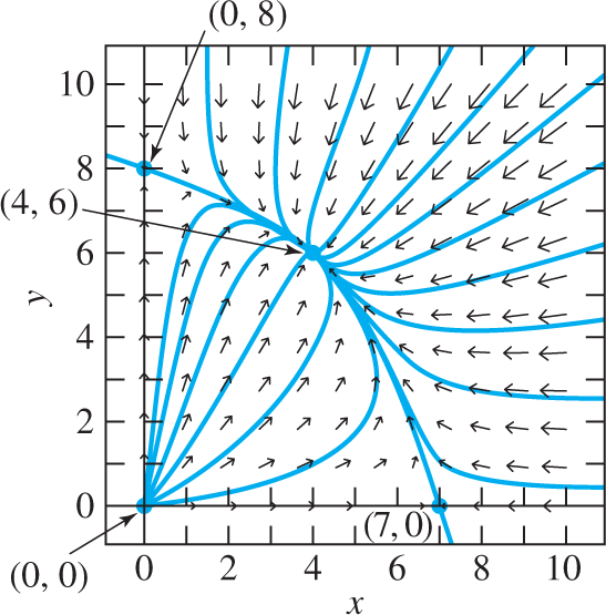
FIGURE 9.3.13.

Direction field and phase portrait for the competition system $x ′ = 14 x - 2 x^{2} - x y, y^{′} = 16 y - 2 y^{2} - x y$ $x ′ = 14 x - 2 x^{2} - x y, y^{′} = 16 y - 2 y^{2} - x y$ of Example 4.

Finally, the interaction between the two populations is one of predation if the interaction coefficients have different signs. For instance, if $c_{1} > 0$ $c_{1} > 0$ but $c_{2} < 0,$ $c_{2} < 0,$ then the x-population is hurt but the y-population is helped by their interaction. We may therefore describe x(t) as a prey population and y(t) as a predator population.

If either $b_{1}$ $b_{1}$ or $b_{2}$ $b_{2}$ is zero in (25), then the corresponding population would (in the absence of the other) exhibit exponential growth rather than logistic growth. For instance, suppose that $a_{1} > 0, a_{2} < 0, b_{1} = b_{2} = 0,$ $a_{1} > 0, a_{2} < 0, b_{1} = b_{2} = 0,$ and $c_{1} > 0, c_{2} < 0 .$ $c_{1} > 0, c_{2} < 0 .$ Then x(t) is a naturally growing prey population while y(t) is a naturally declining predator population. This is the original predator–prey model with which we began this section.

Problems 26 through 34 illustrate a variety of the possibilities indicated here. The problems and examples in this section illustrate the power of elementary critical-point analysis. But remember that ecological systems in nature are seldom so simple as in these examples. Frequently they involve more than two species, and the growth rates of these populations and the interactions among them often are more complicated than those discussed in this section. Consequently, the mathematical modeling of ecological systems remains an active area of current research.

9.3 Problems

Predator–Prey System

Problems 1 and 2 deal with the predator–prey system

\begin{array}{l} \frac{d x}{d t} = 200 x - 4 x y, \\ \frac{d y}{d t} = - 150 y + 2 x y \end{array}

$\begin{array}{l} \frac{d x}{d t} = 200 x - 4 x y, \\ \frac{d y}{d t} = - 150 y + 2 x y \end{array}$ (1)

that corresponds to Fig. 9.3.1.

Starting with the Jacobian matrix of the system in (1), derive its linearizations at the two critical points (0, 0) and (75, 50). Use a graphing calculator or computer system to construct phase plane portraits for these two linearizations that are consistent with the “big picture” shown in Fig. 9.3.1.
Separate the variables in the quotient

$\frac{d y}{d x} = \frac{- 150 y + 2 x y}{200 x - 4 x y}$ $\frac{d y}{d x} = \frac{- 150 y + 2 x y}{200 x - 4 x y}$

of the two equations in (1), and thereby derive the exact implicit solution

$200 \ln y + 150 \ln x - 2 x - 4 y = C$ $200 \ln y + 150 \ln x - 2 x - 4 y = C$

of the system. Use the contour plot facility of a graphing calculator or computer system to plot the contour curves of this equation through the points (75, 100), (75, 150), (75, 200), (75, 250), and (75, 300) in the xy-plane. Are your results consistent with Fig. 9.3.1?
Insect population Let x(t) be a harmful insect population (aphids?) that under natural conditions is held somewhat in check by a benign predator insect population y(t) (ladybugs?). Assume that x(t) and y(t) satisfy the predator–prey equations in (1), so that the stable equilibrium populations are $x_{E} = b / q$ $x_{E} = b / q$ and $y_{E} = a / p .$ $y_{E} = a / p .$ Now suppose that an insecticide is employed that kills (per unit time) the same fraction $f < a$ $f < a$ of each species of insect. Show that the harmful population $x_{E}$ $x_{E}$ is increased, while the benign population $y_{E}$ $y_{E}$ is decreased, so the use of the insecticide is counterproductive. This is an instance in which mathematical analysis reveals undesirable consequences of a well-intentioned interference with nature.

Competition System

Problems 4 through 7 deal with the competition system

\begin{array}{l} \frac{d x}{d t} = 60 x - 4 x^{2} - 3 x y, \\ \frac{d y}{d t} = 42 y - 2 y^{2} - 3 x y, \end{array}

$\begin{array}{l} \frac{d x}{d t} = 60 x - 4 x^{2} - 3 x y, \\ \frac{d y}{d t} = 42 y - 2 y^{2} - 3 x y, \end{array}$ (2)

in which $c_{1} c_{2} = 9 > 8 = b_{1} b_{2},$ $c_{1} c_{2} = 9 > 8 = b_{1} b_{2},$ so the effect of competition should exceed that of inhibition. Problems 4 through 7 imply that the four critical points (0, 0), (0, 21), (15, 0), and (6, 12) of the system in (2) resemble those shown in Fig. 9.3.9—a nodal source at the origin, a nodal sink on each coordinate axis, and a saddle point interior to the first quadrant. In each of these problems use a graphing calculator or computer system to construct a phase plane portrait for the linearization at the indicated critical point. Finally, construct a first-quadrant phase plane portrait for the nonlinear system in (2). Do your local and global portraits look consistent?

Show that the coefficient matrix of the linearization $x ′ = 60 x, y ′ = 42 y$ $x ′ = 60 x, y ′ = 42 y$ of (2) at (0, 0) has positive eigenvalues $λ_{1} = 60$ $λ_{1} = 60$ and $λ_{2} = 42 .$ $λ_{2} = 42 .$ Hence (0, 0) is a nodal source for (2).
Show that the linearization of (2) at (0, 21) is $u ′ = - 3 u, v ′ = - 63 u - 42 v .$ $u ′ = - 3 u, v ′ = - 63 u - 42 v .$ Then show that the coefficient matrix of this linear system has negative eigenvalues $λ_{1} = - 3$ $λ_{1} = - 3$ and $λ_{2} = - 42 .$ $λ_{2} = - 42 .$ Hence (0, 21) is a nodal sink for the system in (2).
Show that the linearization of (2) at (15, 0) is $u ′ = - 60 u - 45 v, v ′ = - 3 v .$ $u ′ = - 60 u - 45 v, v ′ = - 3 v .$ Then show that the coefficient matrix of this linear system has negative eigenvalues $λ_{1} = - 60$ $λ_{1} = - 60$ and $λ_{2} = - 3 .$ $λ_{2} = - 3 .$ Hence (15, 0) is a nodal sink for the system in (2).
Show that the linearization of (2) at (6, 12) is $u ′ = - 24 u - 18 v, v ′ = - 36 u - 24 v .$ $u ′ = - 24 u - 18 v, v ′ = - 36 u - 24 v .$ Then show that the coefficient matrix of this linear system has eigenvalues $λ_{1} = - 24 - 18 \sqrt{2} < 0$ $λ_{1} = - 24 - 18 \sqrt{2} < 0$ and $λ_{2} = - 24 + 18 \sqrt{2} > 0 .$ $λ_{2} = - 24 + 18 \sqrt{2} > 0 .$ Hence (6, 12) is a saddle point for the system in (2).

Competition System

Problems 8 through 10 deal with the competition system

\begin{array}{l} \frac{d x}{d t} = 60 x - 3 x^{2} - 4 x y, \\ \frac{d y}{d t} = 42 y - 3 y^{2} - 2 x y, \end{array}

$\begin{array}{l} \frac{d x}{d t} = 60 x - 3 x^{2} - 4 x y, \\ \frac{d y}{d t} = 42 y - 3 y^{2} - 2 x y, \end{array}$ (3)

in which $c_{1} c_{2} = 8 < 9 = b_{1} b_{2},$ $c_{1} c_{2} = 8 < 9 = b_{1} b_{2},$ so the effect of inhibition should exceed that of competition. The linearization of the system in (3) at (0, 0) is the same as that of (2). This observation and Problems 8 through 10 imply that the four critical points (0, 0), (0, 14), (20, 0), and (12, 6) of (3) resemble those shown in Fig. 9.3.13—a nodal source at the origin, a saddle point on each coordinate axis, and a nodal sink interior to the first quadrant. In each of these problems use a graphing calculator or computer system to construct a phase plane portrait for the linearization at the indicated critical point. Finally, construct a first-quadrant phase plane portrait for the nonlinear system in (3). Do your local and global portraits look consistent?

Show that the linearization of (3) at (0, 14) is $u ′ = 4 u, v ′ = - 28 u - 42 v .$ $u ′ = 4 u, v ′ = - 28 u - 42 v .$ Then show that the coefficient matrix of this linear system has the positive eigenvalue $λ_{1} = 4$ $λ_{1} = 4$ and the negative eigenvalue $λ_{2} = - 42 .$ $λ_{2} = - 42 .$ Hence (0, 14) is a saddle point for the system in (3).
Show that the linearization of (3) at (20, 0) is $u ′ = - 60 u - 80 v, v ′ = 2 v .$ $u ′ = - 60 u - 80 v, v ′ = 2 v .$ Then show that the coefficient matrix of this linear system has the negative eigenvalue $λ_{1} = - 60$ $λ_{1} = - 60$ and the positive eigenvalue $λ_{2} = 2 .$ $λ_{2} = 2 .$ Hence (20, 0) is a saddle point for the system in (3).
Show that the linearization of (3) at (12, 6) is $u ′ = - 36 u - 48 v, v ′ = - 12 u - 18 v .$ $u ′ = - 36 u - 48 v, v ′ = - 12 u - 18 v .$ Then show that the coefficient matrix of this linear system has eigenvalues $λ_{1} = - 27 + 3 \sqrt{73}$ $λ_{1} = - 27 + 3 \sqrt{73}$ and $λ_{2} = - 27 - 3 \sqrt{73},$ $λ_{2} = - 27 - 3 \sqrt{73},$ both of which are negative. Hence (12, 6) is a nodal sink for the system in (3).

Logistic Prey Population

Problems 11 through 13 deal with the predator–prey system

\begin{array}{l} \frac{d x}{d t} = 5 x - x^{2} - x y, \\ \frac{d y}{d t} = - 2 y + x y, \end{array}

$\begin{array}{l} \frac{d x}{d t} = 5 x - x^{2} - x y, \\ \frac{d y}{d t} = - 2 y + x y, \end{array}$ (4)

in which the prey population x(t) is logistic but the predator population y(t) would (in the absence of any prey) decline naturally. Problems 11 through 13 imply that the three critical points (0, 0), (5, 0), and (2, 3) of the system in (4) are as shown in Fig. 9.3.14—with saddle points at the origin and on the positive x-axis, and with a spiral sink interior to the first quadrant. In each of these problems use a graphing calculator or computer system to construct a phase plane portrait for the linearization at the indicated critical point. Do your local portraits look consistent with Fig. 9.3.14?

FIGURE 9.3.14.

Direction field and phase portrait for the predator–prey system of Problems 11 through 13.

Show that the coefficient matrix of the linearization $x ′ = 5 x, y ′ = - 2 y$ $x ′ = 5 x, y ′ = - 2 y$ of (4) at (0, 0) has the positive eigenvalue $λ_{1} = 5$ $λ_{1} = 5$ and the negative eigenvalue $λ_{2} = - 2 .$ $λ_{2} = - 2 .$ Hence (0, 0) is a saddle point of the system in (4).
Show that the linearization of (4) at (5, 0) is $u ′ = - 5 u - 5 v, v ′ = 3 v .$ $u ′ = - 5 u - 5 v, v ′ = 3 v .$ Then show that the coefficient matrix of this linear system has the negative eigenvalue $λ_{1} = - 5$ $λ_{1} = - 5$ and the positive eigenvalue $λ_{2} = 3 .$ $λ_{2} = 3 .$ Hence (5, 0) is a saddle point for the system in (4).
Show that the linearization of (4) at (2, 3) is $u ′ = - 2 u - 2 v, v ′ = 3 u .$ $u ′ = - 2 u - 2 v, v ′ = 3 u .$ Then show that the coefficient matrix of this linear system has the complex conjugate eigenvalues $λ_{1},$ $λ_{1},$ $λ_{2} = - 1 \pm i \sqrt{5}$ $λ_{2} = - 1 \pm i \sqrt{5}$ with negative real part. Hence (2, 3) is a spiral sink for the system in (4).

Doomsday vs. Extinction

Problems 14 through 17 deal with the predator–prey system

\begin{array}{l} \frac{d x}{d t} = x^{2} - 2 x - x y, \\ \frac{d y}{d t} = y^{2} - 4 y + x y . \end{array}

$\begin{array}{l} \frac{d x}{d t} = x^{2} - 2 x - x y, \\ \frac{d y}{d t} = y^{2} - 4 y + x y . \end{array}$ (5)

Here each population—the prey population x(t) and the predator population y(t)—is an unsophisticated population (like the alligators of Section 2.1) for which the only alternatives (in the absence of the other population) are doomsday and extinction. Problems 14 through 17 imply that the four critical points (0, 0), (0, 4), (2, 0), and (3, 1) of the system in (5) are as shown in Fig. 9.3.15—a nodal sink at the origin, a saddle point on each coordinate axis, and a spiral source interior to the first quadrant. This is a two-dimensional version of “doomsday versus extinction.” If the initial point $(x_{0}, y_{0})$ $(x_{0}, y_{0})$ lies in Region I, then both populations increase without bound (until doomsday), whereas if it lies in Region II, then both populations decrease to zero (and thus both become extinct). In each of these problems use a graphing calculator or computer system to construct a phase plane portrait for the linearization at the indicated critical point. Do your local portraits look consistent with Fig. 9.3.15?

FIGURE 9.3.15.

Direction field and phase portrait for the predator–prey system of Problems 14 through 17.

Show that the coefficient matrix of the linearization $x ′ = - 2 x, y ′ = - 4 y$ $x ′ = - 2 x, y ′ = - 4 y$ of the system in (5) at (0, 0) has the negative eigenvalues $λ_{1} = - 2$ $λ_{1} = - 2$ and $λ_{2} = - 4 .$ $λ_{2} = - 4 .$ Hence (0, 0) is a nodal sink for (5).
Show that the linearization of (5) at (0, 4) is $u ′ = - 6 u, v ′ = 4 u + 4 v .$ $u ′ = - 6 u, v ′ = 4 u + 4 v .$ Then show that the coefficient matrix of this linear system has the negative eigenvalue $λ_{1} = - 6$ $λ_{1} = - 6$ and the positive eigenvalue $λ_{2} = 4 .$ $λ_{2} = 4 .$ Hence (0, 4) is a saddle point for the system in (5).
Show that the linearization of (5) at (2, 0) is $u ′ = 2 u - 2 v, v ′ = - 2 v .$ $u ′ = 2 u - 2 v, v ′ = - 2 v .$ Then show that the coefficient matrix of this linear system has the positive eigenvalue $λ_{1} = 2$ $λ_{1} = 2$ and the negative eigenvalue $λ_{2} = - 2 .$ $λ_{2} = - 2 .$ Hence (2, 0) is a saddle point for the system in (5).
Show that the linearization of (5) at (3, 1) is $u ′ = 3 u - 3 v, v ′ = u + v .$ $u ′ = 3 u - 3 v, v ′ = u + v .$ Then show that the coefficient matrix of this linear system has complex conjugate eigenvalues $λ_{1}, λ_{2} = 2 \pm i \sqrt{2}$ $λ_{1}, λ_{2} = 2 \pm i \sqrt{2}$ with positive real part. Hence (3, 1) is a spiral source for (5).

Problems 18 through 25 deal with the predator–prey system

\begin{array}{l} \frac{d x}{d t} = 2 x - x y + ϵ x (5 - x), \\ \frac{d y}{d t} = - 5 y + x y, \end{array}

$\begin{array}{l} \frac{d x}{d t} = 2 x - x y + ϵ x (5 - x), \\ \frac{d y}{d t} = - 5 y + x y, \end{array}$ (6)

for which a bifurcation occurs at the value $ϵ = 0$ $ϵ = 0$ of the parameter $ϵ .$ $ϵ .$ Problems 18 and 19 deal with the case $ϵ = 0,$ $ϵ = 0,$ in which case the system in (6) takes the form

\frac{d x}{d t} = 2 x - x y, \frac{d y}{d t} = - 5 x + x y,

$\frac{d x}{d t} = 2 x - x y, \frac{d y}{d t} = - 5 x + x y,$ (7)

and these problems suggest that the two critical points (0, 0) and (5, 2) of the system in (7) are as shown in Fig. 9.3.16—a saddle point at the origin and a center at (5, 2). In each problem use a graphing calculator or computer system to construct a phase plane portrait for the linearization at the indicated critical point. Do your local portraits look consistent with Fig. 9.3.16?

FIGURE 9.3.16.

The case $ϵ = 0$ $ϵ = 0$ (Problems 18 and 19).

Show that the coefficient matrix of the linearization $x ′ = 2 x, y ′ = - 5 y$ $x ′ = 2 x, y ′ = - 5 y$ of (7) at (0, 0) has the positive eigenvalue $λ_{1} = 2$ $λ_{1} = 2$ and the negative eigenvalue $λ_{2} = - 5 .$ $λ_{2} = - 5 .$ Hence (0, 0) is a saddle point for the system in (7).
Show that the linearization of the system in (7) at (5, 2) is $u ′ = - 5 v, v ′ = 2 u .$ $u ′ = - 5 v, v ′ = 2 u .$ Then show that the coefficient matrix of this linear system has conjugate imaginary eigenvalues $λ_{1},$ $λ_{1},$ $λ_{2} = \pm i \sqrt{10} .$ $λ_{2} = \pm i \sqrt{10} .$ Hence (0, 0) is a stable center for the linear system. Although this is the indeterminate case of Theorem 2 in Section 9.2, Fig. 9.3.16 suggests that (5, 2) also is a stable center for (7).

Problems 20 through 22 deal with the case $ϵ = - 1,$ $ϵ = - 1,$ for which the system in (6) becomes

\frac{d x}{d t} = - 3 x + x^{2} - x y, \frac{d y}{d t} = - 5 y + x y,

$\frac{d x}{d t} = - 3 x + x^{2} - x y, \frac{d y}{d t} = - 5 y + x y,$ (8)

and imply that the three critical points (0, 0), (3, 0), and (5, 2) of (8) are as shown in Fig. 9.3.17—with a nodal sink at the origin, a saddle point on the positive x-axis, and a spiral source at (5, 2). In each problem use a graphing calculator or computer system to construct a phase plane portrait for the linearization at the indicated critical point. Do your local portraits look consistent with Fig. 9.3.17?

FIGURE 9.3.17.

The case $ϵ = - 1$ $ϵ = - 1$ (Problems 20 through 22).

Show that the coefficient matrix of the linearization $x ′ = - 3 x, y ′ = - 5 y$ $x ′ = - 3 x, y ′ = - 5 y$ of the system in (8) at (0, 0) has the negative eigenvalues $λ_{1} = - 3$ $λ_{1} = - 3$ and $λ_{2} = - 5 .$ $λ_{2} = - 5 .$ Hence (0, 0) is a nodal sink for (8).
Show that the linearization of the system in (8) at (3, 0) is $u ′ = 3 u - 3 v, v ′ = - 2 v .$ $u ′ = 3 u - 3 v, v ′ = - 2 v .$ Then show that the coefficient matrix of this linear system has the positive eigenvalue $λ_{1} = 3$ $λ_{1} = 3$ and the negative eigenvalue $λ_{2} = - 2 .$ $λ_{2} = - 2 .$ Hence (3, 0) is a saddle point for (8).
Show that the linearization of (8) at (5, 2) is $u ′ = 5 u - 5 v, v ′ = 2 u .$ $u ′ = 5 u - 5 v, v ′ = 2 u .$ Then show that the coefficient matrix of this linear system has complex conjugate eigenvalues $λ_{1}, λ_{2} = \frac{1}{2} (5 \pm i \sqrt{15})$ $λ_{1}, λ_{2} = \frac{1}{2} (5 \pm i \sqrt{15})$ with positive real part. Hence (5, 2) is a spiral source for the system in (8).

Problems 23 through 25 deal with the case $ϵ = 1,$ $ϵ = 1,$ so that the system in (6) takes the form

\frac{d x}{d t} = 7 x - x^{2} - x y, \frac{d y}{d t} = - 5 y + x y,

$\frac{d x}{d t} = 7 x - x^{2} - x y, \frac{d y}{d t} = - 5 y + x y,$ (9)

and these problems imply that the three critical points (0, 0), (7, 0), and (5, 2) of the system in (9) are as shown in Fig. 9.3.18—with saddle points at the origin and on the positive x-axis and with a spiral sink at (5, 2). In each problem use a graphing calculator or computer system to construct a phase plane portrait for the linearization at the indicated critical point. Do your local portraits look consistent with Fig. 9.3.18?

FIGURE 9.3.18.

The case $ϵ = + 1$ $ϵ = + 1$ (Problems 23 through 25).

Show that the coefficient matrix of the linearization $x ′ = 7 x, y ′ = - 5 y$ $x ′ = 7 x, y ′ = - 5 y$ of (9) at (0, 0) has the positive eigenvalue $λ_{1} = 7$ $λ_{1} = 7$ and the negative eigenvalue $λ_{2} = - 5 .$ $λ_{2} = - 5 .$ Hence (0, 0) is a saddle point for the system in (9).
Show that the linearization of (9) at (7, 0) is $u ′ = - 7 u - 7 v, v ′ = 2 v .$ $u ′ = - 7 u - 7 v, v ′ = 2 v .$ Then show that the coefficient matrix of this linear system has the negative eigenvalue $λ_{1} = - 7$ $λ_{1} = - 7$ and the positive eigenvalue $λ_{2} = 2 .$ $λ_{2} = 2 .$ Hence (7, 0) is a saddle point for the system in (9).
Show that the linearization of (9) at (5, 2) is $u ′ = - 5 u - 5 v, v ′ = 2 u .$ $u ′ = - 5 u - 5 v, v ′ = 2 u .$ Then show that the coefficient matrix of this linear system has the complex conjugate eigenvalues $λ_{1}, λ_{2} = \frac{1}{2} (- 5 \pm i \sqrt{15})$ $λ_{1}, λ_{2} = \frac{1}{2} (- 5 \pm i \sqrt{15})$ with negative real part. Hence (5, 2) is a spiral sink for the system in (9).

For each two-population system in Problems 26 through 34, first describe the type of x- and y-populations involved (exponential or logistic) and the nature of their interaction—competition, cooperation, or predation. Then find and characterize the system’s critical points (as to type and stability). Determine what nonzero x- and y-populations can coexist. Finally, construct a phase plane portrait that enables you to describe the long-term behavior of the two populations in terms of their initial populations x(0) and y(0).

$\frac{d x}{d t} = 2 x - x y, \frac{d y}{d t} = 3 y - x y$ $\frac{d x}{d t} = 2 x - x y, \frac{d y}{d t} = 3 y - x y$
$\frac{d x}{d t} = 2 x y - 4 x, \frac{d y}{d t} = x y - 3 y$ $\frac{d x}{d t} = 2 x y - 4 x, \frac{d y}{d t} = x y - 3 y$
$\frac{d x}{d t} = 2 x y - 16 x, \frac{d y}{d t} = 4 y - x y$ $\frac{d x}{d t} = 2 x y - 16 x, \frac{d y}{d t} = 4 y - x y$
$\frac{d x}{d t} = 3 x - x^{2} - \frac{1}{2} x y, \frac{d y}{d t} = 4 y - 2 x y$ $\frac{d x}{d t} = 3 x - x^{2} - \frac{1}{2} x y, \frac{d y}{d t} = 4 y - 2 x y$
$\frac{d x}{d t} = 3 x - x^{2} + \frac{1}{2} x y, \frac{d y}{d t} = \frac{1}{5} x y - y$ $\frac{d x}{d t} = 3 x - x^{2} + \frac{1}{2} x y, \frac{d y}{d t} = \frac{1}{5} x y - y$
$\frac{d x}{d t} = 3 x - x^{2} - \frac{1}{4} x y, \frac{d y}{d t} = x y - 2 y$ $\frac{d x}{d t} = 3 x - x^{2} - \frac{1}{4} x y, \frac{d y}{d t} = x y - 2 y$
$\frac{d x}{d t} = 30 x - 3 x^{2} + x y, \frac{d y}{d t} = 60 y - 3 y^{2} + 4 x y$ $\frac{d x}{d t} = 30 x - 3 x^{2} + x y, \frac{d y}{d t} = 60 y - 3 y^{2} + 4 x y$
$\frac{d x}{d t} = 30 x - 2 x^{2} - x y, \frac{d y}{d t} = 80 y - 4 y^{2} + 2 x y$ $\frac{d x}{d t} = 30 x - 2 x^{2} - x y, \frac{d y}{d t} = 80 y - 4 y^{2} + 2 x y$
$\frac{d x}{d t} = 30 x - 2 x^{2} - x y, \frac{d y}{d t} = 20 y - 4 y^{2} + 2 x y$ $\frac{d x}{d t} = 30 x - 2 x^{2} - x y, \frac{d y}{d t} = 20 y - 4 y^{2} + 2 x y$

9.3 Application Your Own Wildlife Conservation Preserve

You own a large wildlife conservation preserve that you originally stocked with $F_{0}$ $F_{0}$ foxes and $R_{0}$ $R_{0}$ rabbits on January 1, 2007. The following differential equations model the numbers R(t) of rabbits and F(t) foxes t months later:

\begin{array}{l} \frac{d R}{d t} = (0.01) p R - (0.0001) a R F, \\ \frac{d F}{d t} = - (0.01) q F + (0.0001) b R F, \end{array}

$\begin{array}{l} \frac{d R}{d t} = (0.01) p R - (0.0001) a R F, \\ \frac{d F}{d t} = - (0.01) q F + (0.0001) b R F, \end{array}$

where p and q are the two largest digits (with $p < q$ $p < q$ ) and a and b are the two smallest nonzero digits (with $a < b$ $a < b$ ) in your student ID number.

The numbers of foxes and rabbits will oscillate periodically, out of phase with each other (like the functions x(t) and y(t) in Fig. 9.3.3). Choose your initial numbers $F_{0}$ $F_{0}$ of foxes and $R_{0}$ $R_{0}$ of rabbits—perhaps several hundred of each—so that the resulting solution curve in the RF-plane is a fairly eccentric closed curve. (The eccentricity may be increased if you begin with a relatively large number of rabbits and a small number of foxes, as any wildlife preserve owner would naturally do—because foxes prey on rabbits.)

Your task is to determine

The period of oscillation of the rabbit and fox populations;
The maximum and minimum numbers of rabbits, and the calendar dates on which they first occur;
The maximum and minimum numbers of foxes, and the calendar dates on which they first occur.

With computer software that can plot both RF-trajectories and tR- and tF-solution curves like those in Figs. 9.3.2 and 9.3.3, you can “zoom in” graphically on the points whose coordinates provide the requested information.

..................Content has been hidden....................

You can't read the all page of ebook, please click here login for view all page.

Table of Contents for
9.3 Ecological Models: Predators and Competitors

9.3 Ecological Models: Predators and Competitors

Example 1

FIGURE 9.3.1.

FIGURE 9.3.2.

Example 2

FIGURE 9.3.3.

Competing Species

Example 3

FIGURE 9.3.4.

FIGURE 9.3.5.

FIGURE 9.3.6.

FIGURE 9.3.7.

FIGURE 9.3.8.

FIGURE 9.3.9.

Example 4

FIGURE 9.3.10.

FIGURE 9.3.11.

FIGURE 9.3.12.

Interactions of Logistic Populations

FIGURE 9.3.13.

9.3 Problems

Predator–Prey System

Competition System

Competition System

Logistic Prey Population

FIGURE 9.3.14.

Doomsday vs. Extinction

FIGURE 9.3.15.

FIGURE 9.3.16.

FIGURE 9.3.17.

FIGURE 9.3.18.

9.3 Application Your Own Wildlife Conservation Preserve

Table of Contents for 9.3 Ecological Models: Predators and Competitors

Create new playlist

Sign In

Sign Up

Table of Contents for
9.3 Ecological Models: Predators and Competitors