
9 Nonlinear Systems and Phenomena
9.1 Stability and the Phase Plane
A wide variety of natural phenomena are modeled by two-dimensional first-order systems of the form
![]()
in which the independent variable t does not appear explicitly. We usually think of the dependent variables x and y as position variables in the xy-plane and of t as a time variable. We will see that the absence of t on the right-hand sides in (1) makes the system easier to analyze and its solutions easier to visualize. Using the terminology of Section 2.2, such a system of differential equations in which the derivative values are independent (or “autonomous”) of time t is often called an autonomous system.
We generally assume that the functions F and G are continuously differentiable in some region R of the xy-plane. Then according to the existence and uniqueness theorems of Appendix A, given t0
The equations x=x(t), y=y(t)
If (x⋆,y⋆)
have derivatives x′(t)≡0
In some practical situations these very simple solutions and trajectories are the ones of greatest interest. For example, suppose that the system x′=F(x,y), y′=G(x,y)
Example 1
Find the critical points of the system
Solution
When we look at the equations
that a critical point (x, y) must satisfy, we see that either
and either
If x=0
for x=4, y=6.
Phase Portraits
If the initial point (x0,y0)
Another way of visualizing the system is to construct a slope field in the xy-phase plane by drawing typical line segments having slope
or a direction field by drawing typical vectors pointing the same direction at each point (x, y) as does the vector (F(x, y), G(x, y)). Such a vector field then indicates which direction along a trajectory to travel in order to “go with the flow” described by the system.
Remark
It is worth emphasizing that if our system of differential equations were not autonomous, then its critical points, trajectories, and direction vectors would generally be changing with time. In this event, the concrete visualization afforded by a (fixed) phase portrait or direction field would not be available to us. Indeed, this is a principal reason why an introductory study of nonlinear systems concentrates on autonomous ones.
Figure 9.1.1 shows a direction field and phase portrait for the rabbit-squirrel system of Example 1. The direction field arrows indicate the direction of motion of the point (x(t), y(t)). We see that, given any positive initial numbers x0≠4

FIGURE 9.1.1.
Direction field and phase portrait for the rabbit-squirrel system x′=14x−2x2−xy, y′=16y−2y2−xy
Example 2
For the system
we see from the first equation that x=y

FIGURE 9.1.2.
Direction field for the system in Eq. (7).

FIGURE 9.1.3.
Phase portrait for the system in Eq. (7).
Remark
One could carelessly write the critical points in Example 2 as (±1,±1)
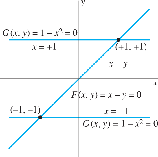
FIGURE 9.1.4.
The two critical points (−1,−1)
Critical Point Behavior
The behavior of the trajectories near an isolated critical point of an autonomous system is of particular interest. Figure 9.1.5 is a close-up view of Fig. 9.1.1 near the critical point (4, 6), and similarly Figs. 9.1.6 and 9.1.7 are close-ups of Fig. 9.1.3 near the critical points (−1,−1)

FIGURE 9.1.5.
Close-up view of Fig. 9.1.1 near the critical point (4, 6).

FIGURE 9.1.6.
Close-up view of Fig. 9.1.3 near the critical point (−1,−1)

FIGURE 9.1.7.
Close-up view of Fig. 9.1.3 near the critical point (1, 1).
These similarities are not a coincidence. Indeed, as we will explore in detail in the next section, the behavior of a nonlinear system near a critical point is generally similar to that of a corresponding linear constant-coefficient system near the origin. For this reason it is useful to extend the language of nodes, sinks, etc., introduced in Section 7.4 for linear constant-coefficient systems to the broader context of critical points of the two-dimensional system (1).
In general, the critical point (x⋆,y⋆)
Either every trajectory approaches (x⋆,y⋆)
(x⋆,y⋆) as t→+∞t→+∞ or every trajectory recedes from (x⋆,y⋆)(x⋆,y⋆) as t→+∞,t→+∞, andEvery trajectory is tangent at (x⋆,y⋆)
(x⋆,y⋆) to some straight line through the critical point.
As with linear constant-coefficient systems, a node is said to be proper provided that no two different pairs of “opposite” trajectories are tangent to the same straight line through the critical point. On the other hand, the critical point (4, 6) of the system in Eq. (5), shown in Figs. 9.1.1 and 9.1.5, is an improper node; as those figures suggest, virtually all of the trajectories approaching this critical point share a common tangent line at that point.
Likewise, a node is further called a sink if all trajectories approach the critical point, a source if all trajectories recede (or emanate) from it. Thus the critical point (4, 6) in Figs. 9.1.1 and 9.1.5 is a nodal sink, whereas the critical point (−1,−1)
Stability
A critical point (x⋆,y⋆)
Thus the critical point x⋆
![]()
for all t>0.
The critical point (x⋆,y⋆)
If (x⋆,y⋆)
It is possible for trajectories to remain near a stable critical point without approaching it, as Example 3 shows.
Example 3
Undamped mass-spring system Consider a mass m that oscillates without damping on a spring with Hooke’s constant k, so that its position function x(t) satisfies the differential equation x″+ω2x=0
with general solution
(10b)
With C=√A2+B2, A=Ccos α,
(11b)
so it becomes clear that each trajectory other than the critical point (0, 0) is an ellipse with equation of the form
As illustrated by the phase portrait in Fig. 9.1.8 (where ω=12

FIGURE 9.1.8.
Direction field and elliptical trajectories for the system x′=y, y′=−14x.
Figure 9.1.9 shows a typical elliptical trajectory in Example 3, with its minor semiaxis denoted by δ

FIGURE 9.1.9.
If the initial point (x0,y0)
Asymptotic Stability
The critical point (x⋆,y⋆)
![]()
where x0=(x0,y0), x⋆=(x⋆,y⋆),
Remark
The stable node shown in Figs. 9.1.1 and 9.1.5 is asymptotically stable because every trajectory approaches the critical point (4, 6) as t→+∞.
Now suppose that x(t) and y(t) denote coexisting populations for which (x⋆,y⋆)
That is, x(t) and y(t) actually approach the equilibrium populations x⋆
For a mechanical system as in Example 3, a critical point represents an equilibrium state of the system—if the velocity y=x′
Moves back toward the equilibrium point as t→+∞
t→+∞ ,Merely remains near the equilibrium point without approaching it, or
Moves farther away from equilibrium.
In Case 1 the critical [equilibrium] point is asymptotically stable; in Case 2 it is stable but not asymptotically so; in Case 3 it is an unstable critical point. A marble balanced on the top of a soccer ball is an example of an unstable critical point. A mass on a spring with damping illustrates the case of asymptotic stability of a mechanical system. The mass-and-spring without damping in Example 3 is an example of a system that is stable but not asymptotically stable.
Example 4
Damped mass-spring system Suppose that m=1
With y=x′
with critical point (0, 0). The characteristic equation r2+2r+2=0
(17b)
where C=√A2+B2

FIGURE 9.1.10.
A stable spiral point and one nearby trajectory.
It is clear from (17) that the point (x(t), y(t)) approaches the origin as t→+∞,
If the arrows in Fig. 9.1.10 were reversed, we would see a trajectory spiraling outward from the origin. An unstable critical point—around which the trajectories spiral as they emanate and recede from it—is called an unstable spiral point (or a spiral source). Example 5 shows that it also is possible for a trajectory to spiral into a closed trajectory—a simple closed solution curve that represents a periodic solution (like the elliptical trajectories in Fig. 9.1.8).
Example 5
Consider the system
In Problem 21 we ask you to show that (0, 0) is its only critical point. This system can be solved explicitly by introducing polar coordinates x=rcos θ, y=rsin θ,
Then substitute the expressions given in (18) for x′
It follows that
Then differentiation of r2=x2+y2
so r=r(t)
In Problem 22 we ask you to derive the solution
where r0=r(0).
If r0=1,

FIGURE 9.1.11.
Spiral trajectories of the system in Eq. (18) with k=5
Under rather general hypotheses it can be shown that there are four possibilities for a nondegenerate trajectory of the autonomous system
The four possibilities are these:
(x(t), y(t)) approaches a critical point as t→+∞
t→+∞ .(x(t), y(t)) is unbounded with increasing t.
(x(t), y(t)) is a periodic solution with a closed trajectory.
(x(t), y(t)) spirals toward a closed trajectory as t→+∞
t→+∞ .
As a consequence, the qualitative nature of the phase plane picture of the trajectories of an autonomous system is determined largely by the locations of its critical points and by the behavior of its trajectories near its critical points. We will see in Section 9.2 that, subject to mild restrictions on the functions F and G, each isolated critical point of the system x′=F(x,y), y′=G(x,y)
9.1 Problems
In Problems 1 through 8, find the critical point or points of the given autonomous system, and thereby match each system with its phase portrait among Figs. 9.1.12 through 9.1.19.
dxdt=2x−y,dydt=x−3y
dxdt=2x−y,dydt=x−3y dxdt=x−y,dydt=x+3y−4
dxdt=x−y,dydt=x+3y−4 dxdt=x−2y+3,dydt=x−y+2
dxdt=x−2y+3,dydt=x−y+2 dxdt=2x−2y−4,dydt=x+4y+3
dxdt=2x−2y−4,dydt=x+4y+3 dxdt=1−y2,dydt=x+2y
dxdt=1−y2,dydt=x+2y dxdt=2−4x−15y,dydt=4−x2
dxdt=2−4x−15y,dydt=4−x2

FIGURE 9.1.12.
Spiral point (−2,1)
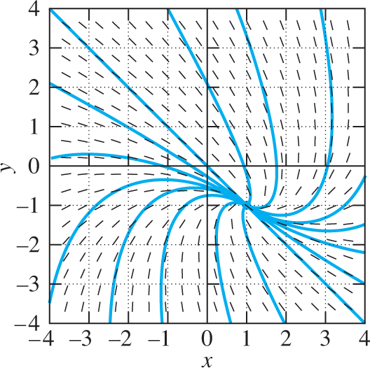
FIGURE 9.1.13.
Spiral point (1,−1)

FIGURE 9.1.14.
Saddle point (0, 0).

FIGURE 9.1.15.
Spiral point (0, 0); saddle points (−2,−1)

FIGURE 9.1.16.
Node (1, 1).

FIGURE 9.1.17.
Spiral point (−1,−1),

FIGURE 9.1.18.
Spiral point (−2,23)

FIGURE 9.1.19.
Stable center (−1,1)
dxdt=x−2y,dydt=4x−x3
dxdt=x−2y,dydt=4x−x3 dxdt=x−y−x2+xy,dydt=−y−x2
dxdt=x−y−x2+xy,dydt=−y−x2
In Problems 9 through 12, find each equilibrium solution x(t)≡x0
x″+4x−x3=0
x''+4x−x3=0 x″+2x′+x+4x3=0
x''+2x'+x+4x3=0 x″+3x′+4sin x=0
x''+3x'+4sin x=0 x″+(x2−1)x′+x=0
x''+(x2−1)x'+x=0
Solve each of the linear systems in Problems 13 through 20 to determine whether the critical point (0, 0) is stable, asymptotically stable, or unstable. Use a computer system or graphing calculator to construct a phase portrait and direction field for the given system. Thereby ascertain the stability or instability of each critical point, and identify it visually as a node, a saddle point, a center, or a spiral point.
dxdt=−2x,dydt=−2y
dxdt=−2x,dydt=−2y dxdt=2x,dydt=−2y
dxdt=2x,dydt=−2y dxdt=−2x,dydt=−y
dxdt=−2x,dydt=−y dxdt=x,dydt=3y
dxdt=x,dydt=3y dxdt=y,dydt=−x
dxdt=y,dydt=−x dxdt=−y,dydt=4x
dxdt=−y,dydt=4x dxdt=2y,dydt=−2x
dxdt=2y,dydt=−2x dxdt=y,dydt=−5x−4y
dxdt=y,dydt=−5x−4y Verify that (0, 0) is the only critical point of the system in Example 6.
In Problems 23 through 26, a system dx/dt=F(x,y), dy/dt=G(x,y)
to find the trajectories of the given system. Use a computer system or graphing calculator to construct a phase portrait and direction field for the system, and thereby identify visually the apparent character and stability of the critical point (0, 0) of the given system.
dxdt=y,dydt=−x
dxdt=y,dydt=−x dxdt=y(1+x2+y2),dydt=x(1+x2+y2)
dxdt=y(1+x2+y2),dydt=x(1+x2+y2) dxdt=4y(1+x2+y2),dydt=−x(1+x2+y2)
dxdt=4y(1+x2+y2),dydt=−x(1+x2+y2) dxdt=y3ex+y,dydt=−x3ex+y
dxdt=y3ex+y,dydt=−x3ex+y Let (x(t), y(t)) be a nontrivial solution of the nonautonomous system
dxdt=y,dydt=tx.dxdt=y,dydt=tx. Suppose that ϕ(t)=x(t+γ)
ϕ(t)=x(t+γ) and ψ(t)=y(t+γ),ψ(t)=y(t+γ), where γ≠0.γ≠0. Show that (ϕ(t),ψ(t))(ϕ(t),ψ(t)) is not a solution of the system.
Problems 28 through 30 deal with the system
in a region where the functions F and G are continuously differentiable, so for each number a and point (x0, y0),
Suppose that (x(t), y(t)) is a solution of the autonomous system and that γ≠0.
γ≠0. Define ϕ(t)=x(t+γ)ϕ(t)=x(t+γ) and ψ(t)=y(t+γ).ψ(t)=y(t+γ). Then show (in contrast with the situation in Problem 27) that (ϕ(t),ψ(t))(ϕ(t),ψ(t)) is also a solution of the system. Thus autonomous systems have the simple but important property that a “t-translate” of a solution is again a solution.Let (x1(t),y1(t))
(x1(t),y1(t)) and (x2(t),y2(t))(x2(t),y2(t)) be two solutions having trajectories that meet at the point (x0,y0)(x0,y0) ; thus x1(a)=x2(b)=x0x1(a)=x2(b)=x0 and y1(a)=y2(b)=y0y1(a)=y2(b)=y0 for some values a and b of t. Definex3(t)=x2(t+γ)andy3(t)=y2(t+γ),x3(t)=x2(t+γ)andy3(t)=y2(t+γ), where γ=b−a,
γ=b−a, so (x2(t),y2(t))(x2(t),y2(t)) and (x3(t),y3(t))(x3(t),y3(t)) have the same trajectory. Apply the uniqueness theorem to show that (x1(t),y1(t))(x1(t),y1(t)) and (x3(t),y3(t))(x3(t),y3(t)) are identical solutions. Hence the original two trajectories are identical. Thus no two different trajectories of an autonomous system can intersect.Suppose that the solution (x1(t),y1(t))
(x1(t),y1(t)) is defined for all t and that its trajectory has an apparent self-intersection:x1(a)=x1(a+P)=x0,y1(a)=y1(a+P)=y0x1(a)=x1(a+P)=x0,y1(a)=y1(a+P)=y0 for some P>0.
P>0. Introduce the solutionx2(t)=x1(t+P),y2(t)=y1(t+P),x2(t)=x1(t+P),y2(t)=y1(t+P), and then apply the uniqueness theorem to show that
x1(t+P)=x1(t)andy1(t)=y1(t+P)x1(t+P)=x1(t)andy1(t)=y1(t+P) for all t. Thus the solution (x1(t),y1(t))
(x1(t),y1(t)) is periodic with period P and has a closed trajectory. Consequently a solution of an autonomous system either is periodic with a closed trajectory, or else its trajectory never passes through the same point twice.
9.1 Application Phase Plane Portraits and First-Order Equations
Consider a first-order differential equation of the form
which may be difficult or impossible to solve explicitly. Its solution curves can nevertheless be plotted as trajectories of the corresponding autonomous two-dimen-sional system
Most ODE plotters can routinely generate phase portraits for autonomous systems. Those appearing in this chapter were plotted using programs that are free for educational use. For instance, the Matlab program pplane illustrated in Fig. 9.1.20 can be found at math.rice.edu/~dfield. Another freely available and user-friendly Matlab-based ODE package with similar graphical capabilities is Iode (www.math.uiuc.edu/iode).

FIGURE 9.1.20.
Matlab pplane menu entries to plot a direction field and phase portrait for the system x′=y,y′=−14x
For example, to plot solution curves for the differential equation
we plot trajectories of the system
The result is shown in Fig. 9.1.21.

FIGURE 9.1.21.
Phase portrait for the system in Eq. (4).
Plot similarly some solution curves for the following differential equations.
dydx=4x−5y2x+3y
dydx=4x−5y2x+3y dydx=4x−5y2x−3y
dydx=4x−5y2x−3y dydx=4x−3y2x−5y
dydx=4x−3y2x−5y dydx=2xyx2−y2
dydx=2xyx2−y2 dydx=x2+2xyy2+2xy
dydx=x2+2xyy2+2xy
Now construct some examples of your own. Homogeneous functions like those in Problems 1 through 5—rational functions with numerator and denominator of the same degree in x and y—work well. The differential equation
of this form generalizes Example 5 in this section but would be inconvenient to solve explicitly. Its phase portrait (Fig. 9.1.22) shows two periodic closed trajectories—the circles r=1

FIGURE 9.1.22.
Phase portrait for the system corresponding to Eq. (5).