Search in book...
Toggle Font Controls
Create new playlist

Name your new playlist

Playlist description (optional)
Sign In

Email address

Password

Forgot Password?

or

Continue with Facebook

Continue with Google
Sign Up

Full Name

Email address

Confirm Email Address

Password

or

Continue with Facebook

Continue with Google

2.6 The Runge–Kutta Method

We now discuss a method for approximating the solution $y = y (x)$ $y = y (x)$ of the initial value problem

\frac{d y}{d x} = f (x, y), y (x_{0}) = y_{0}

$\frac{d y}{d x} = f (x, y), y (x_{0}) = y_{0}$ (1)

that is considerably more accurate than the improved Euler method and is more widely used in practice than any of the numerical methods discussed in Sections 2.4 and 2.5. It is called the Runge–Kutta method, after the German mathematicians who developed it, Carl Runge (1856–1927) and Wilhelm Kutta (1867–1944).

With the usual notation, suppose that we have computed the approximations $y_{1}, y_{2}, y_{3}, \dots, y_{n}$ $y_{1}, y_{2}, y_{3}, \dots, y_{n}$ to the actual values $y (x_{1}), y (x_{2}), y (x_{3}), \dots, y (x_{n})$ $y (x_{1}), y (x_{2}), y (x_{3}), \dots, y (x_{n})$ and now want to compute $y_{n + 1} \approx y (x_{n + 1}) .$ $y_{n + 1} \approx y (x_{n + 1}) .$ Then

y (x_{n + 1}) - y (x_{n}) = \int_{x_{n}}^{x_{n + 1}} y ′ (x) d x = \int_{x_{n}}^{x_{n + h}} y ′ (x) d x

$y (x_{n + 1}) - y (x_{n}) = \int_{x_{n}}^{x_{n + 1}} y ′ (x) d x = \int_{x_{n}}^{x_{n + h}} y ′ (x) d x$ (2)

by the fundamental theorem of calculus. Next, Simpson’s rule for numerical integration yields

y (x_{n + 1}) - y (x_{n}) \approx \frac{h}{6} [y ′ (x_{n}) + 4 y ′ (x_{n} + \frac{h}{2}) + y ′ (x_{n + 1})] .

$y (x_{n + 1}) - y (x_{n}) \approx \frac{h}{6} [y ′ (x_{n}) + 4 y ′ (x_{n} + \frac{h}{2}) + y ′ (x_{n + 1})] .$ (3)

Hence we want to define $y_{n + 1}$ $y_{n + 1}$ so that

y_{n + 1} \approx y_{n} + \frac{h}{6} [y ′ (x_{n}) + 2 y ′ (x_{n} + \frac{h}{2}) + 2 y ′ (x_{n} + \frac{h}{2}) + y ′ (x_{n + 1})];

$y_{n + 1} \approx y_{n} + \frac{h}{6} [y ′ (x_{n}) + 2 y ′ (x_{n} + \frac{h}{2}) + 2 y ′ (x_{n} + \frac{h}{2}) + y ′ (x_{n + 1})];$ (4)

we have split $4 y ′ (x_{n} + \frac{1}{2} h)$ $4 y ′ (x_{n} + \frac{1}{2} h)$ into a sum of two terms because we intend to approximate the slope $y ′ (x_{n} + \frac{1}{2} h)$ $y ′ (x_{n} + \frac{1}{2} h)$ at the midpoint $x_{n} + \frac{1}{2} h$ $x_{n} + \frac{1}{2} h$ of the interval $[x_{n}, x_{n + 1}]$ $[x_{n}, x_{n + 1}]$ in two different ways.

On the right-hand side in (4), we replace the [true] slope values $y ′ (x_{n}), y ′ (x_{n} + \frac{1}{2} h), y ′ (x_{n} + \frac{1}{2} h),$ $y ′ (x_{n}), y ′ (x_{n} + \frac{1}{2} h), y ′ (x_{n} + \frac{1}{2} h),$ and $y ′ (x_{n + 1}),$ $y ′ (x_{n + 1}),$ respectively, with the following estimates.

k_{1} = f (x_{n}, y_{n})

$k_{1} = f (x_{n}, y_{n})$ (5a)

This is the Euler method slope at $x_{n}$ $x_{n}$ .

k_{2} = f (x_{n} + \frac{1}{2} h, y_{n} + \frac{1}{2} h k_{1})

$k_{2} = f (x_{n} + \frac{1}{2} h, y_{n} + \frac{1}{2} h k_{1})$ (5b)

This is an estimate of the slope at the midpoint of the interval $[x_{n}, x_{n + 1}]$ $[x_{n}, x_{n + 1}]$ using the Euler method to predict the ordinate there.

k_{3} = f (x_{n} + \frac{1}{2} h, y_{n} + \frac{1}{2} h k_{2})

$k_{3} = f (x_{n} + \frac{1}{2} h, y_{n} + \frac{1}{2} h k_{2})$ (5c)

This is an improved Euler value for the slope at the midpoint.

k_{4} = f (x_{n + 1}, y_{n} + h k_{3})

$k_{4} = f (x_{n + 1}, y_{n} + h k_{3})$ (5d)

This is the Euler method slope at $x_{n + 1},$ $x_{n + 1},$ using the improved slope $k_{3}$ $k_{3}$ at the midpoint to step to $x_{n + 1}$ $x_{n + 1}$ .

When these substitutions are made in (4), the result is the iterative formula

y_{n + 1} = y_{n} + \frac{h}{6} (k_{1} + 2 k_{2} + 2 k_{3} + k_{4}) .

$y_{n + 1} = y_{n} + \frac{h}{6} (k_{1} + 2 k_{2} + 2 k_{3} + k_{4}) .$ (6)

The use of this formula to compute the approximations $y_{1}, y_{2}, y_{3}, \dots$ $y_{1}, y_{2}, y_{3}, \dots$ successively constitutes the Runge–Kutta method. Note that Eq. (6) takes the “Euler form”

y_{n + 1} = y_{n} + h \cdot k

$y_{n + 1} = y_{n} + h \cdot k$

if we write

k = \frac{1}{6} (k_{1} + 2 k_{2} + 2 k_{3} + k_{4})

$k = \frac{1}{6} (k_{1} + 2 k_{2} + 2 k_{3} + k_{4})$ (7)

for the approximate average slope on the interval $[x_{n}, x_{n + 1}]$ $[x_{n}, x_{n + 1}]$ .

The Runge–Kutta method is a fourth-order method—it can be proved that the cumulative error on a bounded interval [a, b] with $a = x_{0}$ $a = x_{0}$ is of order $h^{4} .$ $h^{4} .$ (Thus the iteration in (6) is sometimes called the fourth-order Runge–Kutta method because it is possible to develop Runge–Kutta methods of other orders.) That is,

| y (x_{n}) - y_{n} | ≦ C h^{4},

$| y (x_{n}) - y_{n} | ≦ C h^{4},$ (8)

where the constant C depends on the function f(x, y) and the interval [a, b], but does not depend on the step size h. The following example illustrates this high accuracy in comparison with the lower-order accuracy of our previous numerical methods.

Example 1

We first apply the Runge–Kutta method to the illustrative initial value problem

\frac{d y}{d x} = x + y, y (0) = 1

$\frac{d y}{d x} = x + y, y (0) = 1$ (9)

that we considered in Fig. 2.4.8 of Section 2.4 and again in Example 2 of Section 2.5. The exact solution of this problem is $y (x) = 2 e^{x} - x - 1 .$ $y (x) = 2 e^{x} - x - 1 .$ To make a point we use $h = 0.5,$ $h = 0.5,$ a larger step size than in any previous example, so only two steps are required to go from $x = 0$ $x = 0$ to $x = 1$ $x = 1$ .

In the first step we use the formulas in (5) and (6) to calculate

\begin{aligned} k_{1} & = & 0 + 1 = 1, \\ k_{2} & = & (0 + 0.25) + (1 + (0.25) \cdot (1)) = 1.5, \\ k_{3} & = & (0 + 0.25) + (1 + (0.25) \cdot (1.5)) = 1.625, \\ k_{4} & = & (0.5) + (1 + (0.5) \cdot (1.625)) = 2.3125, \end{aligned}

$\begin{aligned} k_{1} & = & 0 + 1 = 1, \\ k_{2} & = & (0 + 0.25) + (1 + (0.25) \cdot (1)) = 1.5, \\ k_{3} & = & (0 + 0.25) + (1 + (0.25) \cdot (1.5)) = 1.625, \\ k_{4} & = & (0.5) + (1 + (0.5) \cdot (1.625)) = 2.3125, \end{aligned}$

and then

y_{1} = 1 + \frac{0.5}{6} [1 + 2 \cdot (1.5) + 2 \cdot (1.625) + 2.3125] \approx 1.7969.

$y_{1} = 1 + \frac{0.5}{6} [1 + 2 \cdot (1.5) + 2 \cdot (1.625) + 2.3125] \approx 1.7969.$

Similarly, the second step yields $y_{2} \approx 3.4347$ $y_{2} \approx 3.4347$ .

Figure 2.6.1 presents these results together with the results (from Fig. 2.5.4) of applying the improved Euler method with step size $h = 0.1 .$ $h = 0.1 .$ We see that even with the larger step size, the Runge–Kutta method gives (for this problem) four to five times the accuracy (in terms of relative percentage errors) of the improved Euler method.

FIGURE 2.6.1.

Runge–Kutta and improved Euler results for the initial value problem $d y / d x = x + y, y (0) = 1$ $d y / d x = x + y, y (0) = 1$ .

	Improved Euler		Runge–Kutta
`x`	`y` with $h = 0.1$ $h = 0.1$	Percent Error	`y` with $h = 0.5$ $h = 0.5$	Percent Error	Actual `y`
0.0	1.0000	0.00%	1.0000	0.00%	1.0000
0.5	1.7949	0.14%	1.7969	0.03%	1.7974
1.0	3.4282	0.24%	3.4347	0.05%	3.4366

It is customary to measure the computational labor involved in solving $d y / d x = f (x, y)$ $d y / d x = f (x, y)$ numerically by counting the number of evaluations of the function f(x, y) that are required. In Example 1, the Runge–Kutta method required eight evaluations of $f (x, y) = x + y$ $f (x, y) = x + y$ (four at each step), whereas the improved Euler method required 20 such evaluations (two for each of 10 steps). Thus the Runge–Kutta method gave over four times the accuracy with only 40% of the labor.

Computer programs implementing the Runge–Kutta method are listed in the project material for this section. Figure 2.6.2 shows the results obtained by applying the improved Euler and Runge–Kutta methods to the problem $d y / d x = x + y, y (0) = 1$ $d y / d x = x + y, y (0) = 1$ with the same step size $h = 0.1 .$ $h = 0.1 .$ The relative error in the improved Euler value at $x = 1$ $x = 1$ is about 0.24%, but for the Runge–Kutta value it is 0.00012%. In this comparison the Runge–Kutta method is about 2000 times as accurate, but requires only twice as many function evaluations, as the improved Euler method.

The error bound

| y (x_{n}) - y_{n} | ≦ C h^{4}

$| y (x_{n}) - y_{n} | ≦ C h^{4}$ (8)

for the Runge–Kutta method results in a rapid decrease in the magnitude of errors when the step size h is reduced (except for the possibility that very small step sizes may result in unacceptable roundoff errors). It follows from the inequality in (8) that (on a fixed bounded interval) halving the step size decreases the absolute error by a factor of ${(\frac{1}{2})}^{4} = \frac{1}{16} .$ ${(\frac{1}{2})}^{4} = \frac{1}{16} .$ Consequently, the common practice of successively halving the step size until the computed results “stabilize” is particularly effective with the Runge–Kutta method.

FIGURE 2.6.2.

Runge–Kutta and improved Euler results for the initial value problem $d y / d x = x + y, y (0) = 1,$ $d y / d x = x + y, y (0) = 1,$ with the same step size $h = 0.1.$ $h = 0.1.$

`x`	Improved Euler `y`	Runge–Kutta `y`	Actual `y`
0.1	1.1100	1.110342	1.110342
0.2	1.2421	1.242805	1.242806
0.3	1.3985	1.399717	1.399718
0.4	1.5818	1.583648	1.583649
0.5	1.7949	1.797441	1.797443
0.6	2.0409	2.044236	2.044238
0.7	2.3231	2.327503	2.327505
0.8	2.6456	2.651079	2.651082
0.9	3.0124	3.019203	3.019206
1.0	3.4282	3.436559	3.436564

Example 2

Infinite discontinuity In Example 5 of Section 2.4 we saw that Euler’s method is not adequate to approximate the solution y(x) of the initial value problem

\frac{d y}{d x} = x^{2} + y^{2}, y (0) = 1

$\frac{d y}{d x} = x^{2} + y^{2}, y (0) = 1$ (10)

as x approaches the infinite discontinuity near $x = 0.969811$ $x = 0.969811$ (see Fig. 2.6.3). Now we apply the Runge–Kutta method to this initial value problem.

FIGURE 2.6.3.

Solutions of $d y / d x = x^{2} + y^{2}, y (0) = 1$ $d y / d x = x^{2} + y^{2}, y (0) = 1$ .

Figure 2.6.4 shows Runge–Kutta results on the interval [0.0, 0.9], computed with step sizes $h = 0.1, h = 0.05,$ $h = 0.1, h = 0.05,$ and $h = 0.025 .$ $h = 0.025 .$ There is still some difficulty near $x = 0.9,$ $x = 0.9,$ but it seems safe to conclude from these data that $y (0.5) \approx 2.0670$ $y (0.5) \approx 2.0670$ .

FIGURE 2.6.4.

Approximating the solution of the initial value problem in Eq. (10).

`x`	`y` with $h = 0.1$ $h = 0.1$	`y` with $h = 0.05$ $h = 0.05$	`y` with $h = 0.025$ $h = 0.025$
0.1	1.1115	1.1115	1.1115
0.3	1.4397	1.4397	1.4397
0.5	2.0670	2.0670	2.0670
0.7	3.6522	3.6529	3.6529
0.9	14.0218	14.2712	14.3021

We therefore begin anew and apply the Runge–Kutta method to the initial value problem

\frac{d y}{d x} = x^{2} + y^{2}, y (0.5) = 2.0670.

$\frac{d y}{d x} = x^{2} + y^{2}, y (0.5) = 2.0670.$ (11)

Figure 2.6.5 shows results on the interval [0.5, 0.9], obtained with step sizes $h = 0.01, h = 0.005,$ $h = 0.01, h = 0.005,$ and $h = 0.0025 .$ $h = 0.0025 .$ We now conclude that $y (0.9) \approx 14.3049$ $y (0.9) \approx 14.3049$ .

Finally, Fig. 2.6.6 shows results on the interval [0.90, 0.95] for the initial value problem

\frac{d y}{d x} = x^{2} + y^{2}, y (0.9) = 14.3049,

$\frac{d y}{d x} = x^{2} + y^{2}, y (0.9) = 14.3049,$ (12)

obtained using step sizes $h = 0.002, h = 0.001,$ $h = 0.002, h = 0.001,$ and $h = 0.0005 .$ $h = 0.0005 .$ Our final approximate result is $y (0.95) \approx 50.4723 .$ $y (0.95) \approx 50.4723 .$ The actual value of the solution at $x = 0.95$ $x = 0.95$ is $y (0.95) \approx 50.471867 .$ $y (0.95) \approx 50.471867 .$ Our slight overestimate results mainly from the fact that the four-place initial value in (12) is (in effect) the result of rounding up the actual value $y (0.9) \approx 14.304864;$ $y (0.9) \approx 14.304864;$ such errors are magnified considerably as we approach the vertical asymptote.

FIGURE 2.6.5.

Approximating the solution of the initial value problem in Eq. (11).

`x`	`y` with $h = 0.01$ $h = 0.01$	`y` with $h = 0.005$ $h = 0.005$	`y` with $h = 0.0025$ $h = 0.0025$
0.5	2.0670	2.0670	2.0670
0.6	2.6440	2.6440	2.6440
0.7	3.6529	3.6529	3.6529
0.8	5.8486	5.8486	5.8486
0.9	14.3048	14.3049	14.3049

FIGURE 2.6.6.

Approximating the solution of the initial value problem in Eq. (12).

`x`	`y` with $h = 0.002$ $h = 0.002$	`y` with $h = 0.001$ $h = 0.001$	`y` with $h = 0.0005$ $h = 0.0005$
0.90	14.3049	14.3049	14.3049
0.91	16.7024	16.7024	16.7024
0.92	20.0617	20.0617	20.0617
0.93	25.1073	25.1073	25.1073
0.94	33.5363	33.5363	33.5363
0.95	50.4722	50.4723	50.4723

Example 3

Skydiver A skydiver with a mass of 60 kg jumps from a helicopter hovering at an initial altitude of 5 kilometers. Assume that she falls vertically with initial velocity zero and experiences an upward force $F_{R}$ $F_{R}$ of air resistance given in terms of her velocity v (in meters per second) by

F_{R} = (0.0096) (100 v + 10 v^{2} + v^{3})

$F_{R} = (0.0096) (100 v + 10 v^{2} + v^{3})$

(in newtons, and with the coordinate axis directed downward so that $v > 0$ $v > 0$ during her descent to the ground). If she does not open her parachute, what will be her terminal velocity? How fast will she be falling after 5 s have elapsed? After 10 s? After 20 s?

Solution

Newton’s law $F = m a$ $F = m a$ gives

m \frac{d v}{d t} = m g - F_{R};

$m \frac{d v}{d t} = m g - F_{R};$

that is,

60 \frac{d v}{d t} = (60) (9.8) - (0.0096) (100 v + 10 v^{2} + v^{3})

$60 \frac{d v}{d t} = (60) (9.8) - (0.0096) (100 v + 10 v^{2} + v^{3})$ (13)

because $m = 60$ $m = 60$ and $g = 9.8 .$ $g = 9.8 .$ Thus the velocity function v(t) satisfies the initial value problem

\frac{d v}{d t} = f (v), v (0) = 0,

$\frac{d v}{d t} = f (v), v (0) = 0,$ (14)

where

f (v) = 9.8 - (0.00016) (100 v + 10 v^{2} + v^{3}) .

$f (v) = 9.8 - (0.00016) (100 v + 10 v^{2} + v^{3}) .$ (15)

The skydiver reaches her terminal velocity when the forces of gravity and air resistance balance, so $f (v) = 0 .$ $f (v) = 0 .$ We can therefore calculate her terminal velocity immediately by solving the equation

f (v) = 9.8 - (0.00016) (100 v + 10 v^{2} + v^{3}) = 0.

$f (v) = 9.8 - (0.00016) (100 v + 10 v^{2} + v^{3}) = 0.$ (16)

Figure 2.6.7 shows the graph of the function f(v) and exhibits the single real solution $v \approx 35.5780$ $v \approx 35.5780$ (found graphically or by using a calculator or computer Solve procedure). Thus the skydiver’s terminal speed is approximately 35.578 m/s, about 128 km/h (almost 80 mi/h).

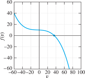
FIGURE 2.6.7.

Graph of $f (v) = 9.8 - (0.00016) (100 v + 10 v^{2} + v^{3}) .$ $f (v) = 9.8 - (0.00016) (100 v + 10 v^{2} + v^{3}) .$

FIGURE 2.6.8.

The skydiver’s velocity data.

`t`(s)	`v`(m/s)
0	0
1	9.636
2	18.386
3	25.299
4	29.949
5	32.678
6	34.137
7	34.875
8	35.239
9	35.415
10	35.500
11	35.541
12	35.560
13	35.569
14	35.574
15	35.576
16	35.577
17	35.578
18	35.578
19	35.578
20	35.578

Figure 2.6.8 shows the results of Runge–Kutta approximations to the solution of the initial value problem in (14); the step sizes $h = 0.2$ $h = 0.2$ and $h = 0.1$ $h = 0.1$ yield the same results (to three decimal places). Observe that the terminal velocity is effectively attained in only 15 s. But the skydiver’s velocity is 91.85% of her terminal velocity after only 5 s, and 99.78% after 10 s.

The final example of this section contains a warning: For certain types of initial value problems, the numerical methods we have discussed are not nearly so successful as in the previous examples.

Example 4

Consider the seemingly innocuous initial value problem

\frac{d y}{d x} = 5 y - 6 e^{- x}, y (0) = 1

$\frac{d y}{d x} = 5 y - 6 e^{- x}, y (0) = 1$ (17)

whose exact solution is $y (x) = e^{- x} .$ $y (x) = e^{- x} .$ The table in Fig. 2.6.9 shows the results obtained by applying the Runge–Kutta method on the interval [0, 4] with step sizes $h = 0.2, h = 0.1,$ $h = 0.2, h = 0.1,$ and $h = 0.05 .$ $h = 0.05 .$ Obviously these attempts are spectacularly unsuccessful. Although $y (x) = e^{- x} \to 0$ $y (x) = e^{- x} \to 0$ as $x \to + \infty,$ $x \to + \infty,$ it appears that our numerical approximations are headed toward $- \infty$ $- \infty$ rather than zero.

FIGURE 2.6.9.

Runge–Kutta attempts to solve numerically the initial value problem in Eq. (17).

`x`	Runge–Kutta `y` with $h = 0.2$ $h = 0.2$	Runge–Kutta `y` with $h = 0.1$ $h = 0.1$	Runge–Kutta `y` with $h = 0.05$ $h = 0.05$	Actual `y`
0.4	0.66880	0.67020	0.67031	0.67032
0.8	0.43713	0.44833	0.44926	0.44933
1.2	0.21099	0.29376	0.30067	0.30119
1.6	$- 0.46019$ $- 0.46019$	0.14697	0.19802	0.20190
2.0	$- 4.72142$ $- 4.72142$	$- 0.27026$ $- 0.27026$	0.10668	0.13534
2.4	$- 35.53415$ $- 35.53415$	$- 2.90419$ $- 2.90419$	$- 0.12102$ $- 0.12102$	0.09072
2.8	$- 261.25023$ $- 261.25023$	$- 22.05352$ $- 22.05352$	$- 1.50367$ $- 1.50367$	0.06081
3.2	$- 1, 916.69395$ $- 1, 916.69395$	$- 163.25077$ $- 163.25077$	$- 11.51868$ $- 11.51868$	0.04076
3.6	$- 14059.35494$ $- 14059.35494$	$- 1205.71249$ $- 1205.71249$	$- 85.38156$ $- 85.38156$	0.02732
4.0	$- 103, 126.5270$ $- 103, 126.5270$	$- 8903.12866$ $- 8903.12866$	$- 631.03934$ $- 631.03934$	0.01832

The explanation lies in the fact that the general solution of the equation $d y / d x = 5 y - 6 e^{- x}$ $d y / d x = 5 y - 6 e^{- x}$ is

y (x) = e^{- x} + C e^{5 x} .

$y (x) = e^{- x} + C e^{5 x} .$ (18)

The particular solution of (17) satisfying the initial condition $y (0) = 1$ $y (0) = 1$ is obtained with $C = 0 .$ $C = 0 .$ But any departure, however small, from the exact solution $y (x) = e^{- x}$ $y (x) = e^{- x}$ —even if due only to roundoff error—introduces [in effect] a nonzero value of C in Eq. (18). And as indicated in Fig. 2.6.10, all solution curves of the form in (18) with $C \neq 0$ $C \neq 0$ diverge rapidly away from the one with $C = 0,$ $C = 0,$ even if their initial values are close to 1.

FIGURE 2.6.10.

Direction field and solution curves for $d y / d x = 5 y - 6 e^{- x} .$ $d y / d x = 5 y - 6 e^{- x} .$

Difficulties of the sort illustrated by Example 4 sometimes are unavoidable, but one can at least hope to recognize such a problem when it appears. Approximate values whose order of magnitude varies with changing step size are a common indicator of such instability. These difficulties are discussed in numerical analysis textbooks and are the subject of current research in the field.

2.6 Problems

A hand-held calculator will suffice for Problems 1 through 10, where an initial value problem and its exact solution are given. Apply the Runge–Kutta method to approximate this solution on the interval [0, 0.5] with step size $h = 0.25 .$ $h = 0.25 .$ Construct a table showing five-decimal-place values of the approximate solution and actual solution at the points $x = 0.25$ $x = 0.25$ and 0.5.

$y ′ = - y,$ $y ′ = - y,$ $y (0) = 2;$ $y (0) = 2;$ $y (x) = 2 e^{- x}$ $y (x) = 2 e^{- x}$
$y ′ = 2 y,$ $y ′ = 2 y,$ $y (0) = \frac{1}{2};$ $y (0) = \frac{1}{2};$ $y (x) = \frac{1}{2} e^{2 x}$ $y (x) = \frac{1}{2} e^{2 x}$
$y ′ = y + 1,$ $y ′ = y + 1,$ $y (0) = 1;$ $y (0) = 1;$ $y (x) = 2 e^{x} - 1$ $y (x) = 2 e^{x} - 1$
$y ′ = x - y,$ $y ′ = x - y,$ $y (0) = 1;$ $y (0) = 1;$ $y (x) = 2 e^{- x} + x - 1$ $y (x) = 2 e^{- x} + x - 1$
$y ′ = y - x - 1,$ $y ′ = y - x - 1,$ $y (0) = 1;$ $y (0) = 1;$ $y (x) = 2 + x - e^{x}$ $y (x) = 2 + x - e^{x}$
$y ′ = - 2 x y,$ $y ′ = - 2 x y,$ $y (0) = 2;$ $y (0) = 2;$ $y (x) = 2 e^{- x^{2}}$ $y (x) = 2 e^{- x^{2}}$
$y ′ = - 3 x^{2} y,$ $y ′ = - 3 x^{2} y,$ $y (0) = 3;$ $y (0) = 3;$ $y (x) = 3 e^{- x^{3}}$ $y (x) = 3 e^{- x^{3}}$
$y ′ = e^{- y},$ $y ′ = e^{- y},$ $y (0) = 0;$ $y (0) = 0;$ $y (x) = \ln (x + 1)$ $y (x) = \ln (x + 1)$
$y ′ = \frac{1}{4} (1 + y^{2}),$ $y ′ = \frac{1}{4} (1 + y^{2}),$ $y (0) = 1;$ $y (0) = 1;$ $y (x) = \tan \frac{1}{4} (x + π)$ $y (x) = \tan \frac{1}{4} (x + π)$
$y ′ = 2 {x y}^{2},$ $y ′ = 2 {x y}^{2},$ $y (0) = 1;$ $y (0) = 1;$ $y (x) = \frac{1}{1 - x^{2}}$ $y (x) = \frac{1}{1 - x^{2}}$

Note: The application following this problem set lists illustrative calculator/computer programs that can be used in the remaining problems.

A programmable calculator or a computer will be useful for Problems 11 through 16. In each problem find the exact solution of the given initial value problem. Then apply the Runge–Kutta method twice to approximate (to five decimal places) this solution on the given interval, first with step size $h = 0.2,$ $h = 0.2,$ then with step size $h = 0.1 .$ $h = 0.1 .$ Make a table showing the approximate values and the actual value, together with the percentage error in the more accurate approximation, for x an integral multiple of 0.2. Throughout, primes denote derivatives with respect to x.

$y ′ = y - 2,$ $y ′ = y - 2,$ $y (0) = 1;$ $y (0) = 1;$ 0 $≦ x ≦ 1$ $≦ x ≦ 1$
$y ′ = \frac{1}{2} {(y - 1)}^{2},$ $y ′ = \frac{1}{2} {(y - 1)}^{2},$ $y (0) = 2;$ $y (0) = 2;$ $0 ≦ x ≦ 1$ $0 ≦ x ≦ 1$
$y y ′ = 2 x^{3},$ $y y ′ = 2 x^{3},$ $y (1) = 3;$ $y (1) = 3;$ $1 ≦ x ≦ 2$ $1 ≦ x ≦ 2$
$x y ′ = y^{2},$ $x y ′ = y^{2},$ $y (1) = 1;$ $y (1) = 1;$ $1 ≦ x ≦ 2$ $1 ≦ x ≦ 2$
$x y ′ = 3 x - 2 y,$ $x y ′ = 3 x - 2 y,$ $y (2) = 3;$ $y (2) = 3;$ $2 ≦ x ≦ 3$ $2 ≦ x ≦ 3$
$y^{2} y ′ = 2 x^{5},$ $y^{2} y ′ = 2 x^{5},$ $y (2) = 3;$ $y (2) = 3;$ $2 ≦ x ≦ 3$ $2 ≦ x ≦ 3$

A computer with a printer is required for Problems 17 through 24. In these initial value problems, use the Runge–Kutta method with step sizes $h = 0.2, 0.1, 0.05,$ $h = 0.2, 0.1, 0.05,$ and 0.025 to approximate to six decimal places the values of the solution at five equally spaced points of the given interval. Print the results in tabular form with appropriate headings to make it easy to gauge the effect of varying the step size h. Throughout, primes denote derivatives with respect to x.

$y ′ = x^{2} + y^{2},$ $y ′ = x^{2} + y^{2},$ $y (0) = 0;$ $y (0) = 0;$ $0 ≦ x ≦ 1$ $0 ≦ x ≦ 1$
$y ′ = x^{2} - y^{2},$ $y ′ = x^{2} - y^{2},$ $y (0) = 1;$ $y (0) = 1;$ $0 ≦ x ≦ 2$ $0 ≦ x ≦ 2$
$y ′ = x + \sqrt{y},$ $y ′ = x + \sqrt{y},$ $y (0) = 1;$ $y (0) = 1;$ $0 ≦ x ≦ 2$ $0 ≦ x ≦ 2$
$y ′ = x + \sqrt[3]{y},$ $y ′ = x + \sqrt[3]{y},$ $y (0) = - 1;$ $y (0) = - 1;$ $0 ≦ x ≦ 2$ $0 ≦ x ≦ 2$
$y ′ = \ln y,$ $y ′ = \ln y,$ $y (1) = 2;$ $y (1) = 2;$ $1 ≦ x ≦ 2$ $1 ≦ x ≦ 2$
$y ′ = x^{2/3} + y^{2/3},$ $y ′ = x^{2/3} + y^{2/3},$ $y (0) = 1;$ $y (0) = 1;$ $0 ≦ x ≦ 2$ $0 ≦ x ≦ 2$
$y ′ = \sin x + \cos y,$ $y ′ = \sin x + \cos y,$ $y (0) = 0;$ $y (0) = 0;$ $0 ≦ x ≦ 1$ $0 ≦ x ≦ 1$
$y ′ = \frac{x}{1 + y^{2}},$ $y ′ = \frac{x}{1 + y^{2}},$ $y (- 1) = 1;$ $y (- 1) = 1;$ $- 1 ≦ x ≦ 1$ $- 1 ≦ x ≦ 1$
Falling parachutist As in Problem 25 of Section 2.5, you bail out of a helicopter and immediately open your parachute, so your downward velocity satisfies the initial value problem

$\frac{d v}{d t} = 32 - 1.6 v, v (0) = 0$ $\frac{d v}{d t} = 32 - 1.6 v, v (0) = 0$

(with t in seconds and v in ft/s). Use the Runge–Kutta method with a programmable calculator or computer to approximate the solution for $0 ≦ t ≦ 2,$ $0 ≦ t ≦ 2,$ first with step size $h = 0.1$ $h = 0.1$ and then with $h = 0.05,$ $h = 0.05,$ rounding off approximate v-values to three decimal places. What percentage of the limiting velocity 20 ft/s has been attained after 1 second? After 2 seconds?
Deer population As in Problem 26 of Section 2.5, suppose the deer population P(t) in a small forest initially numbers 25 and satisfies the logistic equation

$\frac{d P}{d t} = 0.0225 P - 0.0003 P^{2}$ $\frac{d P}{d t} = 0.0225 P - 0.0003 P^{2}$

(with t in months). Use the Runge–Kutta method with a programmable calculator or computer to approximate the solution for 10 years, first with step size $h = 6$ $h = 6$ and then with $h = 3,$ $h = 3,$ rounding off approximate P-values to four decimal places. What percentage of the limiting population of 75 deer has been attained after 5 years? After 10 years?

Use the Runge–Kutta method with a computer system to find the desired solution values in Problems 27 and 28. Start with step size $h = 1,$ $h = 1,$ and then use successively smaller step sizes until successive approximate solution values at $x = 2$ $x = 2$ agree rounded off to five decimal places.

$y ′ = x^{2} + y^{2} - 1, y (0) = 0;$ $y ′ = x^{2} + y^{2} - 1, y (0) = 0;$ $y (2) = ?$ $y (2) = ?$
$y ′ = x + \frac{1}{2} y^{2}, y (- 2) = 0;$ $y ′ = x + \frac{1}{2} y^{2}, y (- 2) = 0;$ $y (2) = ?$ $y (2) = ?$

Velocity-Acceleration Problems

In Problems 29 and 30, the linear acceleration $a = d v / d t$ $a = d v / d t$ of a moving particle is given by a formula $d v / d t = f (t, v),$ $d v / d t = f (t, v),$ where the velocity $v = d y / d t$ $v = d y / d t$ is the derivative of the function $y = y (t)$ $y = y (t)$ giving the position of the particle at time t. Suppose that the velocity v(t) is approximated using the Runge–Kutta method to solve numerically the initial value problem

\frac{d v}{d t} = f (t, v), v (0) = v_{0} .

$\frac{d v}{d t} = f (t, v), v (0) = v_{0} .$ (19)

That is, starting with $t_{0} = 0$ $t_{0} = 0$ and $v_{0},$ $v_{0},$ the formulas in Eqs. (5) and (6) are applied—with t and v in place of x and y—to calculate the successive approximate velocity values $v_{1}, v_{2}, v_{3}, \dots, v_{m}$ $v_{1}, v_{2}, v_{3}, \dots, v_{m}$ at the successive times $t_{1}, t_{2}, t_{3}, \dots, t_{m}$ $t_{1}, t_{2}, t_{3}, \dots, t_{m}$ (with $t_{n + 1} = t_{n} + h$ $t_{n + 1} = t_{n} + h$ ). Now suppose that we also want to approximate the distance y(t) traveled by the particle. We can do this by beginning with the initial position $y (0) = y_{0}$ $y (0) = y_{0}$ and calculating

y_{n + 1} = y_{n} + v_{n} h + \frac{1}{2} a_{n} h^{2}

$y_{n + 1} = y_{n} + v_{n} h + \frac{1}{2} a_{n} h^{2}$ (20)

( $n = 1, 2, 3, \dots$ $n = 1, 2, 3, \dots$ ), where $a_{n} = f (t_{n}, v_{n}) \approx v ′ (t_{n})$ $a_{n} = f (t_{n}, v_{n}) \approx v ′ (t_{n})$ is the particle’s approximate acceleration at time $t_{n} .$ $t_{n} .$ The formula in (20) would give the correct increment (from $y_{n}$ $y_{n}$ to $y_{n + 1}$ $y_{n + 1}$ ) if the acceleration $a_{n}$ $a_{n}$ remained constant during the time interval $[t_{n}, t_{n + 1}]$ $[t_{n}, t_{n + 1}]$ .

Thus, once a table of approximate velocities has been calculated, Eq. (20) provides a simple way to calculate a table of corresponding successive positions. This process is illustrated in the project for this section, by beginning with the velocity data in Fig. 2.6.8 (Example 3) and proceeding to follow the skydiver’s position during her descent to the ground.

Consider again the crossbow bolt of Example 2 in Section 2.3, shot straight upward from the ground with an initial velocity of 49 m/s. Because of linear air resistance, its velocity function $v = d y / d t$ $v = d y / d t$ satisfies the initial value problem

$\frac{d v}{d t} = - (0.04) v - 9.8, v (0) = 49$ $\frac{d v}{d t} = - (0.04) v - 9.8, v (0) = 49$

with exact solution $v (t) = 294 e^{- t / 25} - 245 .$ $v (t) = 294 e^{- t / 25} - 245 .$ (a) Use a calculator or computer implementation of the Runge–Kutta method to approximate v(t) for $0 ≦ t ≦ 10$ $0 ≦ t ≦ 10$ using both $n = 100$ $n = 100$ and $n = 200$ $n = 200$ subintervals. Display the results at intervals of 1 second. Do the two approximations—each rounded to four decimal places—agree both with each other and with the exact solution? (b) Now use the velocity data from part (a) to approximate y(t) for $0 ≦ t ≦ 10$ $0 ≦ t ≦ 10$ using $n = 200$ $n = 200$ subintervals. Display the results at intervals of 1 second. Do these approximate position values—each rounded to two decimal places—agree with the exact solution

$y (t) = 7350 (1 - e^{- t / 25}) - 245 t ?$ $y (t) = 7350 (1 - e^{- t / 25}) - 245 t ?$

(c) If the exact solution were unavailable, explain how you could use the Runge–Kutta method to approximate closely the bolt’s times of ascent and descent and the maximum height it attains.
Now consider again the crossbow bolt of Example 3 in Section 2.3. It still is shot straight upward from the ground with an initial velocity of 49 m/s, but because of air resistance proportional to the square of its velocity, its velocity function v(t) satisfies the initial value problem

$\frac{d v}{d t} = - (0.0011) v | v | - 9.8, v (0) = 49.$ $\frac{d v}{d t} = - (0.0011) v | v | - 9.8, v (0) = 49.$

Beginning with this initial value problem, repeat parts (a) through (c) of Problem 29 (except that you may need $n = 200$ $n = 200$ subintervals to get four-place accuracy in part (a) and $n = 400$ $n = 400$ subintervals for two-place accuracy in part (b)). According to the results of Problems 17 and 18 in Section 2.3, the bolt’s velocity and position functions during ascent and descent are given by the following formulas.

$\begin{array}{l} Ascent: \\ \begin{aligned} v (t) & = & (94.388) \tan (0.478837 - [0.103827] t), \\ y (t) & = & 108.465 \\ + (909.091) \ln (\cos (0.478837 - [0.103827] t)); \end{aligned} \\ Descent: \\ \begin{aligned} v (t) & = & - (94.388) \tanh (0.103827 [t - 4.6119]), \\ y (t) & = & 108.465 \\ - (909.091) \ln (\cosh (0.103827 [t - 4.6119])) . \end{aligned} \end{array}$ $\begin{array}{l} Ascent: \\ \begin{aligned} v (t) & = & (94.388) \tan (0.478837 - [0.103827] t), \\ y (t) & = & 108.465 \\ + (909.091) \ln (\cos (0.478837 - [0.103827] t)); \end{aligned} \\ Descent: \\ \begin{aligned} v (t) & = & - (94.388) \tanh (0.103827 [t - 4.6119]), \\ y (t) & = & 108.465 \\ - (909.091) \ln (\cosh (0.103827 [t - 4.6119])) . \end{aligned} \end{array}$

2.6 Application Runge–Kutta Implementation

Figure 2.6.11 lists TI-Nspire CX CAS and Python programs implementing the Runge–Kutta method to approximate the solution of the initial value problem

\frac{d y}{d x} = x + y, y (0) = 1

$\frac{d y}{d x} = x + y, y (0) = 1$

considered in Example 1 of this section. The comments provided in the final column should make these programs intelligible even if you have little familiarity with the Python and TI programming languages.

To apply the Runge–Kutta method to a different equation $d y / d x = f (x, y),$ $d y / d x = f (x, y),$ one need only change the initial line of the program, in which the function f is defined. To increase the number of steps (and thereby decrease the step size), one need only change the value of n specified in the second line of the program.

Figure 2.6.12 exhibits a Matlab implementation of the Runge–Kutta method. Suppose that the function f describing the differential equation $y ′ = f (x, y)$ $y ′ = f (x, y)$ has been defined. Then the rk function takes as input the initial value x, the initial value y, the final value x1 of x, and the desired number n of subintervals. As output it produces the resulting column vectors x and y of x- and y-values. For instance, the Matlab command

FIGURE 2.6.11.

TI-Nspire CX CAS and Python Runge–Kutta programs.

TI-Nspire CX CAS Python Comment

TI-Nspire CX CAS	Python	Comment
`Define rk()=Prgm f(x,y):=x+y n:=10 x:=0.0 y:=1.0 x1:=1.0 h:=(x1-x)/n For i,1,n x0:=x y0:=y k1:=f(x,y) x:=x0+h/2 y:=y0+(hk1)/2 k2:=f(x,y) y:=y0+(hk2)/2 k3:=f(x,y) x:=x0+h y:=y0+hk3 k4:=f(x,y) k:=(k1+2k2+2k3+k4)/6 y:=y0+hk Disp x,y EndFor EndPrgm`	`# Program RK def F(X,Y): return X + Y N = 10 X = 0.0 Y = 1.0 X1 = 1.0 H = (X1-X)/N for I in range(N): X0 = X Y0 = Y K1 = F(X,Y) X = X0 + H/2 Y = Y0 + HK1/2 K2 = F(X,Y) Y = Y0 + HK2/2 K3 = F(X,Y) X = X0 + H Y = Y0 + HK3 K4 = F(X,Y) K = (K1+2K2+2K3 +K4)/6 Y = Y0 + HK print (X,Y) # END`	`Program title Define function f No. of steps Initial x Initial y Final x Step size Begin loop Save previous x Save previous y First slope Midpoint Midpt predictor Second slope Midpt predictor Third slope New x Endpt predictor Fourth slope Average slope Corrector Display results End loop`

Define rk()=Prgm
    f(x,y):=x+y
    n:=10
    x:=0.0
    y:=1.0
    x1:=1.0
    h:=(x1-x)/n
    For i,1,n
       x0:=x
       y0:=y
       k1:=f(x,y)
       x:=x0+h/2
       y:=y0+(h*k1)/2
       k2:=f(x,y)
       y:=y0+(h*k2)/2
       k3:=f(x,y)
       x:=x0+h
       y:=y0+h*k3
       k4:=f(x,y)
       k:=(k1+2*k2+2*k3+k4)/6
       y:=y0+h*k
       Disp x,y
    EndFor
EndPrgm

# Program RK
def F(X,Y): return X + Y
N = 10
X = 0.0
Y = 1.0
X1 = 1.0
H = (X1-X)/N
for I in range(N):
X0 = X
Y0 = Y
K1 = F(X,Y)
X = X0 + H/2
Y = Y0 + H*K1/2
K2 = F(X,Y)
Y = Y0 + H*K2/2
K3 = F(X,Y)
X = X0 + H
Y = Y0 + H*K3
K4 = F(X,Y)
K = (K1+2*K2+2*K3
  +K4)/6
Y = Y0 + H*K
print (X,Y)
# END

Program title
Define function f
No. of steps
Initial x
Initial y
Final x
Step size
Begin loop
Save previous x
Save previous y
First slope
Midpoint
Midpt predictor
Second slope
Midpt predictor
Third slope
New x
Endpt predictor
Fourth slope
Average slope
Corrector
Display results
End loop

function yp = f(x,y)
yp = x + y;                          % yp = y’
function [X,Y] = rk(x,y,x1,n)
h = (x1 - x)/n;                      % step size
X = x;                               % initial x
Y = y;                               % initial y
for i = 1:n                          % begin loop
    k1 = f(x,y);                     % first slope
    k2 = f(x+h/2,y+h*k1/2);          % second slope
    k3 = f(x+h/2,y+h*k2/2);          % third slope
    k4 = f(x+h,y+h*k3);              % fourth slope
    k  = (k1+2*k2+2*k3+k4)/6;        % average slope
    x  = x + h;                      % new x
    y  = y + h*k;                    % new y
    X  = [X;x];                      % update x-column
    Y  = [Y;y];                      % update y-column
    end                              % end loop

FIGURE 2.6.12.

Matlab implementation of the Runge–Kutta method.

[X, Y] = rk(0, 1, 1, 10)

then generates the first and third columns of data shown in the table in Fig. 2.6.2.

You should begin this project by implementing the Runge–Kutta method with your own calculator or computer system. Test your program by applying it first to the initial value problem in Example 1, then to some of the problems for this section.

Famous Numbers Revisited, One Last Time

The following problems describe the numbers

e \approx 2.71828182846, \ln 2 \approx 0.69314718056, and π \approx 3.14159265359

$e \approx 2.71828182846, \ln 2 \approx 0.69314718056, and π \approx 3.14159265359$

as specific values of certain initial value problems. In each case, apply the Runge–Kutta method with $n = 10, 20, 40, \dots$ $n = 10, 20, 40, \dots$ subintervals (doubling n each time). How many subintervals are needed to obtain-twice in succession-the correct value of the target number rounded to nine decimal places?

The number $e = y (1),$ $e = y (1),$ where y(x) is the solution of the initial value problem $d y / d x = y, y (0) = 1$ $d y / d x = y, y (0) = 1$ .
The number $\ln 2 = y (2),$ $\ln 2 = y (2),$ where y(x) is the solution of the initial value problem $d y / d x = 1 / x, y (1) = 0$ $d y / d x = 1 / x, y (1) = 0$ .
The number $π = y (1),$ $π = y (1),$ where y(x) is the solution of the initial value problem $d y / d x = 4 / (1 + x^{2}), y (0) = 0$ $d y / d x = 4 / (1 + x^{2}), y (0) = 0$ .

The Skydiver’s Descent

The following Matlab function describes the skydiver’s acceleration function in Example 3.

function  vp = f(t,v)
vp = 9.8 - 0.00016*(100*v + 10*v^2 + v^3);

Then the commands

k = 200                      % 200 subintervals
[t,v] = rk(0, 0, 20, k);     % Runge–Kutta approximation
[t(1:10:k+1); v(1:10:k+1)]   % Display every 10th entry

produce the table of approximate velocities shown in Fig. 2.6.8. Finally, the commands

y = zeros(k+1,1):                       % initialize y
h = 0.1;                                % step size
for n = 1:k                             % for n = 1 to k
  a = f(t(n),v(n)):                     % acceleration
  y(n+1) = y(n) + v(n)*h +0.5*a*h^2;    % Equation (20)
end                                     % end loop
[t(1:20:k+1),v(1:20:k+1),y(1:20:k+1)]   % each 20th entry

carry out the position function calculations described in Eq. (20) in the instructions for Problems 29 and 30. The results of these calculations are shown in the table in Fig. 2.6.13. It appears that the skydiver falls 629.866 m during her first 20 s of descent, and then free falls the remaining 4370.134 meters to the ground at her terminal speed of 35.578 m/s. Hence her total time of descent is $20 + (4370.134/35.578) \approx 142.833$ $20 + (4370.134/35.578) \approx 142.833$ s, or about 2 min 23 s.

FIGURE 2.6.13.

The skydiver’s velocity and position data.

`t` (s)	`v` (m/s)	`y` (m)
0	0	0
2	18.386	18.984
4	29.949	68.825
6	34.137	133.763
8	35.239	203.392
10	35.500	274.192
12	35.560	345.266
14	35.574	416.403
16	35.577	487.555
18	35.578	558.710
20	35.578	629.866

For an individual problem to solve after implementing these methods using an available computer system, analyze your own skydive (perhaps from a different height), using your own mass m and a plausible air-resistance force of the form $F_{R} = a v + {b v}^{2} + {c v}^{3}$ $F_{R} = a v + {b v}^{2} + {c v}^{3}$ .

..................Content has been hidden....................

You can't read the all page of ebook, please click here login for view all page.

Table of Contents for 2.6 The Runge&#8211;Kutta Method The Runge–Kutta Method

Create new playlist

Sign In

Sign Up

Table of Contents for
2.6 The Runge–Kutta Method The Runge–Kutta Method