
2.2 Equilibrium Solutions and Stability
In previous sections we have often used explicit solutions of differential equations to answer specific numerical questions. But even when a given differential equation is difficult or impossible to solve explicitly, it often is possible to extract qualitative information about general properties of its solutions. For example, we may be able to establish that every solution x(t) grows without bound as t→+∞,
Example 1
Cooling and heating Let x(t) denote the temperature of a body with initial temperature x(0)=x0.
we readily solve (by separation of variables) for the explicit solution
It follows immediately that
so the temperature of the body approaches that of the surrounding medium (as is evident to one’s intuition). Note that the constant function x(t)≡A
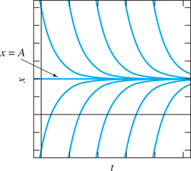
FIGURE 2.2.1.
Typical solution curves for the equation of Newton’s law of cooling, dx/dt=−k(x−A)
Remark
The behavior of solutions of Eq. (1) is summarized briefly by the phase diagram in Fig. 2.2.2—which indicates the direction (or “phase”) of change in x as a function of x itself. The right-hand side f(x)=−k(x−A)=k(A−x)

FIGURE 2.2.2.
Phase diagram for the equation dx/dt=f(x)=k(A−x)
In Section 2.1 we introduced the general population equation
where β
This is an autonomous first-order differential equation—one in which the independent variable t does not appear explicitly (the terminology here stemming from the Greek word autonomos for “independent,” e.g., of the time t). As in Example 1, the solutions of the equation f(x)=0
If x=c
Example 2 illustrates the fact that the qualitative behavior (as t increases) of the solutions of an autonomous first-order equation can be described in terms of its critical points.
Example 2
Logistic equation Consider the logistic differential equation
(with k>0
In Section 2.1 we discussed the logistic-equation solution
satisfying the initial condition x(0)=x0.
We observed in Section 2.1 that if x0>0,
Because the numerator in (6) is negative in this case, it follows that
It follows that the solution curves of the logistic equation in (5) look as illustrated in Fig. 2.2.3. Here we see graphically that every solution either approaches the equilibrium solution x(t)≡M
Stability of Critical Points
Figure 2.2.3 illustrates the concept of stability. A critical point x=c
for all t>0.

FIGURE 2.2.3.
Typical solution curves for the logistic equation dx/dt=kx(M−x)
Figure 2.2.4 shows a “wider view” of the solution curves of a logistic equation with k=1

FIGURE 2.2.4.
Solution curves, funnel, and spout for dx/dt=4x−x2
Remark 1
We can summarize the behavior of solutions of the logistic equation in (5)—in terms of their initial values—by means of the phase diagram shown in Fig. 2.2.5. It indicates that x(t)→M

FIGURE 2.2.5.
Phase diagram for the logistic equation dx/dt=f(x)=kx(M−x)
Remark 2
Related to the stability of the limiting solution M=a/b
is the “predictability” of M for an actual population. The coefficients a and b are unlikely to be known precisely for an actual population. But if they are replaced with close approximations a⋆
Example 3
Explosion/extinction Consider now the explosion/extinction equation
of Eq. (10) in Section 2.1. Like the logistic equation, it has the two critical points x=0
(with only a single difference in sign from the logistic solution in (6)). If x0<M,
Because the numerator in (10) is positive in this case, it follows that
Therefore, the solution curves of the explosion/extinction equation in (9) look as illustrated in Fig. 2.2.6. A narrow band along the equilibrium curve x=0

FIGURE 2.2.6.
Typical solution curves for the explosion/extinction equation dx/dt=kx(x−M)
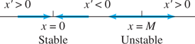
FIGURE 2.2.7.
Phase diagram for the explosion/extinction equation dx/dt=f(x)=kx(x−M)
Harvesting a Logistic Population
The autonomous differential equation
(with a, b, and h all positive) may be considered to describe a logistic population with harvesting. For instance, we might think of the population of fish in a lake from which h fish per year are removed by fishing.
Example 4
Threshold/limiting population Let us rewrite Eq. (11) in the form
which exhibits the limiting population M in the case h=0
assuming that the harvesting rate h is sufficiently small that 4h<kM2,
For instance, the number of critical points of the equation may change abruptly as the value of a parameter is changed. In Problem 24 we ask you to solve this equation for the solution
in terms of the initial value x(0)=x0
Note that the exponent −k(N−H)t
In Problem 25 we ask you to deduce also from Eq. (15) that
for a positive value t1
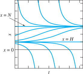
FIGURE 2.2.8.
Typical solution curves for the logistic harvesting equation dx/dt=k(N−x)(x−H).

FIGURE 2.2.9.
Phase diagram for the logistic harvesting equation dx/dt=f(x)=k(N−x)(x−H).
Example 5
Lake stocked with fish For a concrete application of our stability conclusions in Example 4, suppose that k=1
has solutions H=1
Bifurcation and Dependence on Parameters
A biological or physical system that is modeled by a differential equation may depend crucially on the numerical values of certain coefficients or parameters that appear in the equation. For instance, the number of critical points of the equation may change abruptly as the value of a parameter is changed.
Example 6
Critical/excessive harvesting The differential equation
(with x in hundreds) models the harvesting of a logistic population with k=1
Now let’s investigate the dependence of this picture upon the harvesting level h. According to Eq. (13) with k=1
If h<4
But if h=4,

FIGURE 2.2.10.
Solution curves of the equation x′=x(4−x)−h
If, finally, h>4,

FIGURE 2.2.11.
Solution curves of the equation x′=x(4−x)−h
If we imagine turning a dial to gradually increase the value of the parameter h in Eq. (19), then the picture of the solution curves changes from one like Fig. 2.2.8 with h<4,
two critical points if h<4
h<4 ;one critical point if h=4
h=4 ;no critical point if h>4
h>4 .
The value h=4
where either c=N

FIGURE 2.2.12.
The parabola (c−2)2=4−h
2.2 Problems
In Problems 1 through 12 first solve the equation f(x)=0
dxdt=x−4
dxdt=x−4 dxdt=3−x
dxdt=3−x dxdt=x2−4x
dxdt=x2−4x dxdt=3x−x2
dxdt=3x−x2 dxdt=x2−4
dxdt=x2−4 dxdt=9−x2
dxdt=9−x2 dxdt=(x−2)2
dxdt=(x−2)2 dxdt=−(3−x)2
dxdt=−(3−x)2 dxdt=x2−5x+4
dxdt=x2−5x+4 dxdt=7x−x2−10
dxdt=7x−x2−10 dxdt=(x−1)3
dxdt=(x−1)3 dxdt=(2−x)3
dxdt=(2−x)3
In Problems 13 through 18, use a computer system or graphing calculator to plot a slope field and/or enough solution curves to indicate the stability or instability of each critical point of the given differential equation. (Some of these critical points may be semistable in the sense mentioned in Example 6.)
dxdt=(x+2)(x−2)2
dxdt=(x+2)(x−2)2 dxdt=x(x2−4)
dxdt=x(x2−4) dxdt=(x2−4)2
dxdt=(x2−4)2 dxdt=(x2−4)3
dxdt=(x2−4)3 dxdt=x2(x2−4)
dxdt=x2(x2−4) dxdt=x3(x2−4)
dxdt=x3(x2−4) The differential equation dx/dt=110x(10−x)−h
dx/dt=110x(10−x)−h models a logistic population with harvesting at rate h. Determine (as in Example 6) the dependence of the number of critical points on the parameter h, and then construct a bifurcation diagram like Fig. 2.2.12.The differential equation dx/dt=1100x(x−5)+s
dx/dt=1100x(x−5)+s models a population with stocking at rate s. Determine the dependence of the number of critical points c on the parameter s, and then construct the corresponding bifurcation diagram in the sc-plane.Pitchfork bifurcation Consider the differential equation dx/dt=kx−x3.
dx/dt=kx−x3. (a) If k≦0,k≦0, show that the only critical value c=0c=0 of x is stable. (b) If k>0,k>0, show that the critical point c=0c=0 is now unstable, but that the critical points c=±√kc=±k−−√ are stable. Thus the qualitative nature of the solutions changes at k=0k=0 as the parameter k increases, and so k=0k=0 is a bifurcation point for the differential equation with parameter k. The plot of all points of the form (k, c) where c is a critical point of the equation x′=kx−x3x'=kx−x3 is the “pitchfork diagram” shown in Fig. 2.2.13.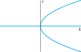
FIGURE 2.2.13.
Bifurcation diagram for dx/dt=kx−x3
dx/dt=kx−x3 .Consider the differential equation dx/dt=x+kx3
dx/dt=x+kx3 containing the parameter k. Analyze (as in Problem 21) the dependence of the number and nature of the critical points on the value of k, and construct the corresponding bifurcation diagram.Variable-rate harvesting Suppose that the logistic equation dx/dt=kx(M−x)
dx/dt=kx(M−x) models a population x(t) of fish in a lake after t months during which no fishing occurs. Now suppose that, because of fishing, fish are removed from the lake at the rate of hxhx fish per month (with h a positive constant). Thus fish are “harvested” at a rate proportional to the existing fish population, rather than at the constant rate of Example 4. (a) If 0<h<kM,0<h<kM, show that the population is still logistic. What is the new limiting population? (b) If h≧kM,h≧kM, show that x(t)→0x(t)→0 are t→+∞,t→+∞, so the lake is eventually fished out.Separate variables in the logistic harvesting equation dx/dt=k(N−x)(x−H)
dx/dt=k(N−x)(x−H) and then use partial fractions to derive the solution given in Eq. (15).Use the alternative forms
x(t)=N(x0 − H) + H(N − x0)e − k(N − H)t(x0 − H) + (N − x0)e − k(N − H)t=H(N − x0)e − k(N − H)t − N(H − x0)(N − x0)e − k(N − H)t − (H − x0)x(t)==N(x0 − H) + H(N − x0)e − k(N − H)t(x0 − H) + (N − x0)e − k(N − H)tH(N − x0)e − k(N − H)t − N(H − x0)(N − x0)e − k(N − H)t − (H − x0) of the solution in (15) to establish the conclusions stated in (17) and (18).
Constant-Rate Harvesting
Example 4 dealt with the case 4h>kM2
If 4h=kM2,
4h=kM2, show that typical solution curves look as illustrated in Fig. 2.2.14. Thus if x0≧M/2,x0≧M/2, then x(t)→M/2x(t)→M/2 as t→+∞.t→+∞. But if x0<M/2,x0<M/2, then x(t)=0x(t)=0 after a finite period of time, so the lake is fished out. The critical point x=M/2x=M/2 might be called semistable, because it looks stable from one side, unstable from the other.
FIGURE 2.2.14.
Solution curves for harvesting a logistic population with 4h=kM2
4h=kM2 .If 4h>kM2,
4h>kM2, show that x(t)=0x(t)=0 after a finite period of time, so the lake is fished out (whatever the initial population). [Suggestion: Complete the square to rewrite the differential equation in the form dx/dt=−k[(x−a)2+b2].dx/dt=−k[(x−a)2+b2]. Then solve explicitly by separation of variables.] The results of this and the previous problem (together with Example 4) show that h=14kM2h=14kM2 is a critical harvesting rate for a logistic population. At any lesser harvesting rate the population approaches a limiting population N that is less than M (why?), whereas at any greater harvesting rate the population reaches extinction.Alligator population This problem deals with the differential equation dx/dt=kx(x−M)−h
dx/dt=kx(x−M)−h that models the harvesting of an unsophisticated population (such as alligators). Show that this equation can be rewritten in the form dx/dt=k(x−H)(x−K),dx/dt=k(x−H)(x−K), whereH=12(M+√M2+4h/k)>0,K=12(M−√M2+4h/k)<0.HK==12(M+M2+4h/k−−−−−−−−−√)>0,12(M−M2+4h/k−−−−−−−−−√)<0. Show that typical solution curves look as illustrated in Fig. 2.2.15.
Consider the two differential equations
dxdt=(x−a)(x−b)(x−c)(21)dxdt=(x−a)(x−b)(x−c) anddxdt=(a−x)(b−x)(c−x),(22)anddxdt=(a−x)(b−x)(c−x), each having the critical points a, b, and c; suppose that a<b<c.
a<b<c. For one of these equations, only the critical point b is stable; for the other equation, b is the only unstable critical point. Construct phase diagrams for the two equations to determine which is which. Without attempting to solve either equation explicitly, make rough sketches of typical solution curves for each. You should see two funnels and a spout in one case, two spouts and a funnel in the other.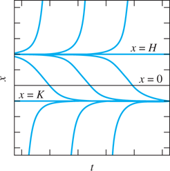
FIGURE 2.2.15.
Solution curves for harvesting a population of alligators.