
10.3 Translation and Partial Fractions
As illustrated by Examples 1 and 2 of Section 10.2, the solution of a linear differential equation with constant coefficients can often be reduced to the matter of finding the inverse Laplace transform of a rational function of the form
where the degree of P(s) is less than that of Q(s). The technique for finding is based on the same method of partial fractions that we use in elementary calculus to integrate rational functions. The following two rules describe the partial fraction decomposition of R(s), in terms of the factorization of the denominator Q(s) into linear factors and irreducible quadratic factors corresponding to the real and complex zeros, respectively, of Q(s).
Finding involves two steps. First we must find the partial fraction decomposition of R(s), and then we must find the inverse Laplace transform of each of the individual partial fractions of the types that appear in (2) and (3). The latter step is based on the following elementary property of Laplace transforms.
Proof:
If we simply replace s with in the definition of we obtain
If we apply the translation theorem to the formulas for the Laplace transforms of and that we already know—multiplying each of these functions by and replacing s with in the transforms—we get the following additions to the table in Fig. 10.1.2.
| f(t) | F(s) | ||
|---|---|---|---|
| (6) | |||
| (7) | |||
| (8) |
For ready reference, all the Laplace transforms derived in this chapter are listed in the table of transforms that appears in the endpapers.

FIGURE 10.3.1.
The mass–spring–dashpot system of Example 1.
Example 1
Damped mass-spring system Consider a mass-and-spring system with and in mks units (Fig. 10.3.1). As usual, let x(t) denote the displacement of the mass m from its equilibrium position. If the mass is set in motion with and find x(t) for the resulting damped free oscillations.
Solution
The differential equation is so we need to solve the initial value problem
We take the Laplace transform of each term of the differential equation. Because (obviously) we get the equation
which we solve for
Applying the formulas in (7) and (8) with and we now see that
Figure 10.3.2 shows the graph of this rapidly decaying damped oscillation.
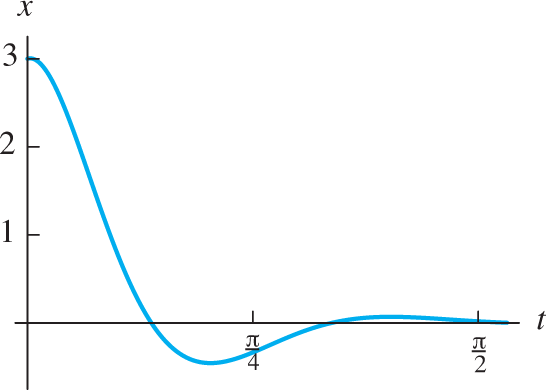
FIGURE 10.3.2.
The position function x(t) in Example 1.
Example 2 illustrates a useful technique for finding the partial fraction coefficients in the case of nonrepeated linear factors.
Example 2
Find the inverse Laplace transform of
Solution
Note that the denominator of R(s) factors as Hence
Multiplication of each term of this equation by Q(s) yields
When we successively substitute the three zeros and of the denominator Q(s) in this equation, we get the results
Thus and so
and therefore
Example 3 illustrates a differentiation technique for finding the partial fraction coefficients in the case of repeated linear factors.
Example 3
Solve the initial value problem
Solution
The transformed equation is
Thus
To find A, B, and C, we multiply both sides by to obtain
where is the sum of the two partial fractions corresponding to Substitution of in Eq. (10) yields To find B and C, we differentiate Eq. (10) twice to obtain
and
Now substitution of in Eq. (11) yields and substitution of in Eq. (12) yields .
To find D and E, we multiply each side in Eq. (9) by to get
where and then differentiate to obtain
Substitution of in Eqs. (13) and (14) now yields and Thus
so the solution of the given initial value problem is
Examples 4, 5, and 6 illustrate techniques for dealing with quadratic factors in partial fraction decompositions.
Example 4
Mass–spring–dashpot system Consider the mass–spring–dashpot system as in Example 1, but with initial conditions and with the imposed external force Find the resulting transient motion and steady periodic motion of the mass.
Solution
The initial value problem we need to solve is
The transformed equation is
Hence
When we multiply both sides by the common denominator, we get
To find A and B, we substitute the zero of the quadratic factor in Eq. (15); the result is
which we simplify to
We now equate real parts and imaginary parts on each side of this equation to obtain the two linear equations
which are readily solved for and .
To find C and D, we substitute the zero of the quadratic factor in Eq. (15) and get
which we simplify to
Again we equate real parts and imaginary parts; this yields the two linear equations
and we readily find their solution to be .
With these values of the coefficients A, B, C, and D, our partial fractions decomposition of X(s) is
After we compute the inverse Laplace transforms, we get the position function
The terms of circular frequency 2 constitute the steady periodic forced oscillation of the mass, whereas the exponentially damped terms of circular frequency 5 constitute its transient motion, which disappears very rapidly (see Fig. 10.3.3). Note that the transient motion is nonzero even though both initial conditions are zero.

FIGURE 10.3.3.
The periodic forced oscillation damped transient motion and solution in Example 4.
Resonance and Repeated Quadratic Factors
The following two inverse Laplace transforms are useful in inverting partial fractions that correspond to the case of repeated quadratic factors:
These follow from Example 5 and Problem 31 of Section 10.2, respectively. Because of the presence in Eqs. (16) and (17) of the terms and a repeated quadratic factor ordinarily signals the phenomenon of resonance in an undamped mechanical or electrical system.
Example 5
Use Laplace transforms to solve the initial value problem
that determines the undamped forced oscillations of a mass on a spring.
Solution
When we transform the differential equation, we get the equation
If we find without difficulty that
so it follows that
But if we have
so Eq. (17) yields the resonance solution
Remark
The solution curve defined in Eq. (18) bounces back and forth (see Fig. 10.3.4) between the “envelope curves” that are obtained by writing (18) in the form
and then defining the usual “amplitude” In this case we find that
This technique for constructing envelope curves of resonance solutions is illustrated further in the application material for this section.
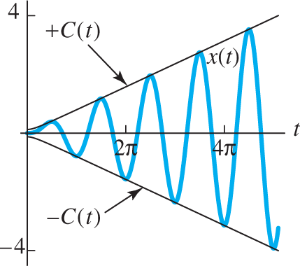
FIGURE 10.3.4.
The resonance solution in (18) with and together with its envelope curves
Example 6
Solve the initial value problem
Solution
First we observe that
Hence the transformed equation is
Thus our problem is to find the inverse transform of
If we multiply by the common denominator we get the equation
Upon substituting we find that .
Equation (20) is an identity that holds for all values of s. To find the values of the remaining coefficients, we substitute in succession the values and in Eq. (20). This yields the system
of five linear equations in B, C, D, E, and F. With the aid of a calculator programmed to solve linear systems, we find that and .
We now substitute in Eq. (19) the coefficients we have found, and thus obtain
Recalling Eq. (16), the translation property, and the familiar transforms of and we see finally that the solution of the given initial value problem is
10.3 Problems
Apply the translation theorem to find the Laplace transforms of the functions in Problems 1 through 4.
Apply the translation theorem to find the inverse Laplace transforms of the functions in Problems 5 through 10.
Use partial fractions to find the inverse Laplace transforms of the functions in Problems 11 through 22.
Use the factorization
to derive the inverse Laplace transforms listed in Problems 23 through 26.
Use Laplace transforms to solve the initial value problems in Problems 27 through 38.
Resonance
Problems 39 and 40 illustrate two types of resonance in a mass–spring–dashpot system with given external force F(t) and with the initial conditions .
Suppose that and Use the inverse transform given in Eq. (16) to derive the solution Construct a figure that illustrates the resonance that occurs.
Suppose that and Derive the solution
Show that the maximum value of the amplitude function is Thus (as indicated in Fig. 10.3.5) the oscillations of the mass increase in amplitude during the first 5 s before being damped out as .

FIGURE 10.3.5.
The graph of the damped oscillation in Problem 40.
10.3 Application Damping and Resonance Investigations
Here we outline a Maple investigation of the behavior of the mass–spring–dashpot system
with parameter values
m := 25; c := 10; k := 226;in response to a variety of possible external forces:
This should give damped oscillations “leveling off” to a constant solution (why?).
With this periodic external force you should see a steady periodic oscillation with an exponentially damped transient motion (as illustrated in Fig. 5.6.13).
Now the periodic external force is exponentially damped, and the transform X(s) includes a repeated quadratic factor that signals the presence of a resonance phenomenon. The response x(t) isa constant multiple of that shown in Fig. 10.3.5.
We have inserted the factor t to make it a bit more interesting. The solution in this case is illustrated below.
In this case you’ll find that the transform X(s) involves the fifth power of a quadratic factor, and its inverse transform by manual methods would be impossibly tedious.
To illustrate the Maple approach, we first set up the differential equation corresponding to Case 4.
F := 900*t*exp(t/5) *cos(3* t);
de := m* diff(x(t),t$2) + c* diff(x(t),t) + k* x(t) = F;
Then we apply the Laplace transform and substitute the initial conditions.
with(inttrans):
DE := laplace(de, t, s):
X(s) := solve(DE, laplace(x(t), t, s)):
X(s) := simplify(subs(x(0)=0, D(x)(0)=0, X(s)));
At this point the command factor(denom(X(s))) shows that
The cubed quadratic factor would be difficult to handle manually, but the command
x(t) := invlaplace(X(s), s, t);soon yields
The amplitude function for these damped oscillations is defined by
C(t) := exp(-t/5)*sqrt(t^2 + (3*t^2 1/3)^2);and finally the command
plot({x(t), C(t), -C(t)}, t=0..40);produces the plot shown in Fig. 10.3.6. The resonance resulting from the repeated quadratic factor consists of a temporary buildup before the oscillations are damped out.

FIGURE 10.3.6.
The resonance solution and its envelope curves in Case 4.
For a similar solution in one of the other cases listed previously, you need only enter the appropriate force F in the initial command above and then re-execute the subsequent commands. To see the advantage of using Laplace transforms, set up the differential equation de for Case 5 and examine the result of the command
dsolve({de, x(0)=0, D(x)(0)=0}, x(t));Of course you can substitute your own favorite mass–spring–dashpot parameters for those used here. But it will simplify the calculations if you choose m, c, and k so that
where p, a, and b are integers. One way is to select the latter integers first, then use Eq. (2) to determine m, c, and k.