1.5 Book's Organization

This book is organized in accordance with the order laid out by seven parts in three categories presented in the previous section. Each part can be read independently while keeping sufficient correlation with other parts.

1.5.1 Part I: Preliminaries

The preliminaries in Part I help readers grasp sufficient knowledge to follow this book without difficulty. It consists of six chapters.

Chapter 2 is Fundamentals of Subsample and Mixed Sample Analyses. It uses a simple example to illustrate issues of subsamples and mixed samples encountered in detection and classification. It then walks through various approaches using hard and soft decisions for subsample detection and mixed sample classification. It includes many techniques currently being used and available in the literature.

Chapter 3 introduces Three-Dimensional Receiver Operating Characteristics (3D ROC) Analysis that can be used as an evaluation tool for soft decision-making performance for hyperspectral target detection and classification. An ROC curve is defined as a curve plotted based on detection probability versus false alarm probability. An analysis that uses ROC curves to evaluate the effectiveness of a Neyman–Pearson detector is called ROC analysis. A major advantage of ROC analysis is that there is no need of specifying a particular cost function. For example, least squares error or signal-to-noise ratio may be a good criterion for detection of problems in signal processing and communications, but may not be appropriate to measure image quality or classification accuracy. This is essentially true when it comes to design of computer-aided diagnostic systems where their effectiveness is measured by their end users in which case the cost function is generally human errors. Furthermore, ROC analysis is developed for detection in the context of binary hypothesis testing problems. In chemical/biological warfare (CBW) defense, estimation of chemical/biological (CB) agent abundance is more critical than CB agent detection since the lethal level of concentration of different CB agents poses different threats. The detection-based ROC curves cannot address this need. Chapter 3 is included to resolve this issue where a 3D ROC analysis is developed by creating a third dimension to specify target abundance so that a 3D-ROC curve can be generated and plotted based on three parameters, detection probability, P_D, false alarm probability, P_F, and threshold τ. Consequently, the traditional detection-based ROC curves, referred to as 2D ROC curves, become a special case of 3D ROC curves. As noted, most hyperspectral imaging techniques are actually derived from various aspects of estimation, which produce abundance fractions of signatures of interest such as linear spectral mixture analysis. In order to evaluate their performance for quantitative analysis the estimated abundance fractions must be converted to hard decisions via a threshold τ. The 3D ROC analysis provides a feasible tool for this purpose.

Chapter 4 is Design of Synthetic Image Experiments. One of major difficulties in algorithm design is how to evaluate various algorithms objectively and impartially on a fair common ground. In doing so, the first concern is the data to be used for experiments that must be available and assessable for those who are interested in comparing their designed algorithms to others. This can be done by using data sets in the public domain. A second concern is that the experiments should be repeatable for performance assessment. A third and most important one is design of experiments that should have controllable parameters to generate desired ground truth to address issues to be investigated. Chapter 4 takes advantage of real image scenes available on web site to simulate synthetic images with various scenarios that can be designed for this purpose.

Chapter 5 is Virtual Dimensionality of Hyperspectral Data that revisits a recently developed concept called virtual dimensionality defined in Chapter 17 of Chang (2003a) as the number of spectrally distinct signatures in hyperspectral imagery. VD has been found to be very useful in many applications (Chang, 2006a, 2006b) such as DR in Wang and Chang (2006a), BS in Chang and Wang (2006), and endmember extraction in Wang and Chang (2006b). Accordingly, a new way of reinterpreting VD becomes imperative. Chapter 5 is a result of such an effort where VD is explored for new interpretation and various techniques are also developed to estimate VD for different applications.

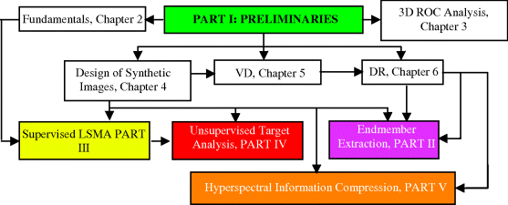
Chapter 6 is Data Dimensionality Reduction. It provides a comprehensive study and survey on many popular and commonly used dimensionality reduction (DR) techniques, which can be treated in two separate categories: dimensionality reduction by transform (DRT) and DR by band selection (DRBS). Specifically, DRT comprises two types of transforms: component analysis (CA)-based transforms, which are derived from statistics of various orders including 2nd order statistics-based principal components analysis (PCA), 3rd order statistics-based skewness, 4th order statistics-based kurtosis and statistical independency-based independent component analysis (ICA) and feature extraction (FE)-based transforms, Fisher's ratio-based linear discriminant analysis (FLDA), and linear mixture model-based OSP. As an alternative to DRT, DRBS selects an appropriate subset of bands from the original band set to replace the high-dimensional original data set with a low-dimensional data set represented by selected bands. So, technically speaking, DRBS performs data reduction, not data compression, by reducing band dimensionality without processing data in the sense that selected bands form a new data cube with all the unselected bands being discarded. While both DRT and DRBS accomplish the same goal, they present different rationales in DR. The former is developed to compact data information in low dimensions via a transform, while the latter represents the original high-dimensional data by its low-dimensional data via band selection. As a consequence, the effectiveness of DR and BS is measured by the transform used for DR and criteria used for BS. Nevertheless, DRT and DRBS do share the same fundamental issue, that is, “how many dimensions are required to be retained after DRT?” and “how many bands are needed for DRBS to faithfully represent the original data?.” Interestingly, such an issue has been either overlooked or intentionally avoided in the past because finding an effective criterion for determination of the number of dimensions to be retained or bands to be selected is extremely challenging. Figure 1.1 lists six chapters in Part I to provide background knowledge for follow-up chapters.

Figure 1.1 Six chapters in Part I to provide background knowledge.

1.5.2 Part II: Endmember Extraction

Endmembers are probably one of most important features in hyperspectral data exploitation since they represent pure signatures used to specify distinct spectral classes. So, finding endmembers becomes a very crucial preprocessing step for hyperspectral image analysis. This is particularly true for linear spectral mixture analysis (LSMA) that requires a set of basic material constituents, referred to as image endmembers to form a linear mixing model to unmix data in terms of abundance fractions of these endmembers. However, the prior knowledge of such image endmembers is usually not available a priori. Therefore, endmember extraction comes to play a key role in finding such image endmembers. Unfortunately, the research in endmember extraction has not received much attention in early days until recently. This may be partly due to the fact that many research efforts in remote sensing image processing have been directed to design and development of supervised methods where the necessary prior knowledge is assumed provided a priori. In this case, there is no need of finding endmembers. Second, because of low spectral or spatial resolution most image pixels appear in a mixed form rather than as pure pixels. Consequently, the presence of endmembers is considered to be very rare. From a land use/land cover's point of view there may be few endmembers that have little impact on image classification. However, from a viewpoint of intelligence endmembers provide crucial and critical information since their existence is unexpected. Specifically, when they appear, only a small population will be present and cannot be identified by prior knowledge. Additionally, the low probability of their occurrence also makes their detection very difficult. Part II is devoted to this topic. Most importantly, it develops various algorithms of different forms for endmember extraction.

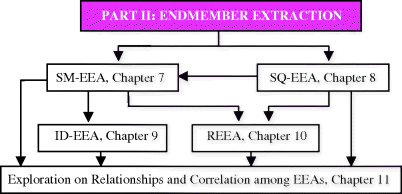
Basically, an endmember extraction algorithm (EEA) can be categorized into simultaneous EEA (SM-EEA) and sequential EAA (SQ-EEA) depending upon how it generates endmembers. An SM-EEA generates a required number of endmembers all together compared to an SQ-EEA, which generates one endmember at a time until it reaches a required number of endmembers. On the other hand, based on how initial conditions are used for initialization, an EEA can be also categorized into initialization-driven EEA (ID-EEA) and random EEA (REEA). These two types of EEAs adopt completely opposite philosophies. An ID-EEA selects a specific set of initial endmembers to avoid randomness caused by the use of random initial endmembers compared to an REEA, which converts the disadvantage resulting from random nature of initial endmembers to an advantage of making an EEA immune to random initial conditions. In order to treat EEAs systematically and logically, Chapter 7 first considers SM-EEAs followed by SQ-EEAs in Chapter 8, ID-EEAs in Chapter 9, and REEA in Chapter 10. Finally, Part II is concluded by Chapter 11, which explores relationships among various EEAs studied in Chapters 7–10. Figure 1.2 outlines the organization of five chapters in Part II.

Figure 1.2 Organization of five chapters in Part II.

1.5.3 Part III: Supervised Linear Hyperspectral Mixture Analysis

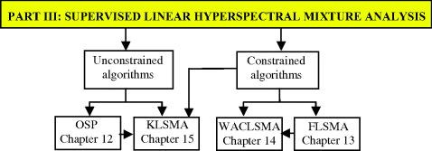
Supervised linear hyperspectral mixture analysis (SLSMA) is probably the most widely used hyperspectral imaging technique to perform various tasks for data analysis. It makes an assumption that a data sample vector can be described by a linear mixing model as a linear mixture of a finite number of known basic signature constituents called image endmembers, from which it can be unmixed via a specific linear spectral unmixing technique into abundance fractions of these image endmembers. Since SLSMA has been previously treated in the book by Chang (2003a), the five chapters, Chapters 12–15 presented in this book, can be considered as an expansion of SLSMA and complement to the LSMA discussed in Chang (2003a). Chapter 12 revisits the orthogonal subspace projection originally developed by Harsanyi and Chang (1994). In particular, when only partial knowledge such as desired target information is provided with no prior background knowledge, OSP can be implemented as the constrained energy minimization developed in Harsanyi's dissertation (1993). If no prior knowledge is available, then OSP can be implemented as RX detector (Reed and Yu, 1990) for anomaly detection. Chapter 13 presents a third approach to SLSMA, Fisher's linear spectral mixture analysis (FLSMA), which replaces the signal-to-noise ratio criterion used by OSP or least squares error (LSE) used by LSOSP with the criterion of Fisher's ratio. Chapter 14 further extends OSP and FLSMA to WAC-LSMA by replacing the commonly used LSE with weighted LSE. While Chapters 13 and 14 extend SLSMA via imposing constraints on the used linear mixing model, Chapter 15 derives kernel-based LSMA, which extends SLSMA techniques to their kernel-based counterparts via nonlinear functions. Figure 1.3 outlines the organization of four chapters in Part III.

Figure 1.3 Organization of four chapters in Part III.

1.5.4 Part IV: Unsupervised Hyperspectral Analysis

One of major tasks in hyperspectral imaging is target detection and classification. Due to its high spectral resolution, targets of interest are generally different from those in multispectral imagery. For example, endmembers and anomalies that generally do not contribute much to land cover/land use classification are actually crucial in hyperspectral image analysis. Other targets of interest in hyperspectral data analysis also include rare minerals in geology, special spices in agriculture and ecology, drug trafficking in law enforcement, combat vehicles in battlefield, man-made targets in intelligent analysis, and so on. Realistically, most of such targets generally appear as either mixed pixels or subpixels. So, the major goal of Part IV is to extend the SLSMA in Part III to ULSMA where two main issues that do not occur in the SLSMA need to be addressed in ULSMA. One is the number of signature sources of interest, p. The other is how to find these signature sources once the value of the p is determined. Since the first issue can be addressed by the concept of VD developed in Chapter 5, the main theme of Part IV is primarily focused on the second issue.

Chapter 16 investigates two types of hyperspectral measures: signature-based and correlation-weighted measures, both of which can be used to discriminate and identify unknown signature vectors for unsupervised data analysis. The former includes the spectral angle mapper (SAM), Euclidean distance, spectral information divergence (SID), and orthogonal projection divergence (OPD), while the latter uses the sample spectral correlation as a weighting factor to measure signature similarity for discrimination and identification.

Chapter 17 extends SLSMA to ULSMA. In doing so, two approaches are developed to find unknown image endmembers, referred to as virtual signatures (VSs). The first one is to implement LSMA techniques in an unsupervised manner on the original data and its sphered data to find two sets of VSs corresponding to background and target signatures, respectively. A second approach is to use components analysis methods where PCA and ICA are implemented to find unknown background and target signatures, respectively.

Due to substantial amount of information provided by hundreds of contiguous spectral bands it is interesting to know how much information can be extracted from a single hyperspectral image pixel vector as well as how to process the extracted pixel information for data analysis. In traditional image processing the only image pixel information is uniquely specified by its gray-level value. In multispectral image processing with only tens of discrete spectral bands in use, the spectral information provided by a multispectral image pixel is generally very limited compared to that provided by a hyperspectral image pixel. So, the issue in exploration of information extraction from a single hyperspectral image pixel vector has not received much interest as it should. Very little work has been done in the past. For example, an endmember itself provides vital information of a particular spectral class. Another example is an anomaly that provides information in identifying unknown targets. While an endmember is specifically defined, the definition of anomaly seems vague with a general understanding that an anomaly is a target whose spectral signature is distinct from those of pixels in its surrounding neighborhood. However, how large should a surrounding neighborhood be for a pixel vector to be qualified as anomalous pixel vector? So far, there is no answer to it. More generally, for a given pixel vector, how can we characterize the pixel vector as a subpixel vector or a mixed pixel vector or an anomalous pixel vector or a pixel vector of some other type? Besides, can an endmember be a pure pixel vector, in which case it is referred to as endmember pixel vector or vice versa? Can a pixel be both an anomalous pixel vector and an endmember pixel vector? As a complete opposite to anomaly, how can we view a pixel vector if the spectral signatures of pixel vectors in its proximity are very similar and close to each other? Interestingly, these issues have never been investigated on a single pixel vector basis. So, Chapter 18 investigates the issue of “what spectral information can be extracted from a single hyperspectral image pixel vector?” Figure 1.4 outlines the organization of two chapters in Part IV.

Figure 1.4 Organization of three chapters in Part IV.

1.5.5 Part V: Hyperspectral Information Compression

Data compression has received increasing interest in hyperspectral data analysis because of the vast amount of data volumes needed to be processed and significant redundancy resulting from high interband spectral correlation. Since a hyperspectral image can be viewed as a 3D image cube, a common practice is a direct application of 3D compression techniques available in image/video processing to hyperspectral imagery so as to achieve so-called hyperspectral data compression. Unfortunately, there are several issues arising from such an approach. One is how to deal with spectral compression from very high spectral resolution provided by a hyperspectral imaging sensor. The reason why the hyperspectral imagery is called “hyperspectral” is due to its wealthy spectral information, which offers unique spectral characterization that cannot be provided by spatial information, particularly, the spectral profile information provided by subpixels and mixed pixels across its acquired wavelength range by hundreds of spectral channels. Therefore, from a hyperspectral imagery point of view, spectral information is usually more important and crucial than spatial information when it comes to hyperspectral image analysts. When hyperspectral compression is performed, extra care must be taken of in order to preserve spectral characteristics and properties. For example, when targets of interest are rare such as anomalies and endmembers, their spatial extent is generally very small and limited. Thus, the spatial correlation resulting from such targets will be too little to be used for spatial compression. In this case a direct spatial compression without taking into account spectral properties of these targets may result in significant loss of information that characterizes these targets. As a consequence, blindly applying 3D compression techniques to hyperspectral data may not be able to achieve effective compression from an exploitation perspective. Accordingly, a more appropriate approach is to consider “information” compression rather than “data” compression since the compression is performed based on preservation of the information of interest instead of reduction in data size. More specifically, an effective technique in compressing data size does not necessarily imply that it is also effective in compressing information to be retained. To resolve this dilemma, an effective means of compressing hyperspectral imagery may be one that performs compression in a two-stage process that carries out spectral compression in the first stage to preserve crucial spectral information to avoid being compromised by the follow-up spatial compression in the second stage (Ramakrishna et al., 2005a, 2005b). Such a two-stage compression is referred to as hyperspectral information compression or exploitation-based lossy hyperspectral data compression in this book as opposed to lossy hyperspectral data compression, commonly referred in the literature. Five chapters are presented in Part V and outlined in Figure 1.5.

Figure 1.5 Organization of three chapters in Part V.

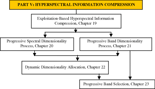
Chapter 19 reviews issues arising in data compression commonly used in the literature and further introduces a new concept of hyperspectral information compression or exploitation-based lossy hyperspectral data compression where various approaches can be derived for different applications in data exploitation. This chapter is followed by two new approaches to hyperspectral information compression developed in Chapters 20 and 21, which develop techniques to process spectral dimensions and band dimensions in a progressive manner, referred to as progressive spectral dimensionality process (PSDP) and progressive band dimensionality process (PBDP), respectively. In order to more effectively determine spectral and band dimensionality to be used for material classification Chapter 22 presents a new idea of dynamic dimensionality allocation (DDA). By taking advantage of PBDP in Chapter 21 and DDA in Chapter 22 a new approach to band selection, called progressive band selection (PBS), is further developed and presented in Chapter 23.

1.5.6 Part VI: Hyperspectral Signal Coding

So far, data processing discussed in all the previous chapters, Chapters 7–23, is considered as hyperspectral image processing because the considered data are image data cubes and the techniques are developed to process hyperspectral data as an image cube with data samples treated as image pixel vectors. However, due to the use of hundreds of spectral channels a hyperspectral data sample vector already contains spectral information that can be used for data analysis without relying on sample spectral correlation provided by image structures. So, instead of considering a data sample vector as an image pixel vector in an image cube, a data sample vector can also be processed as a one-dimensional signal, referred to as a hyperspectral signal or signature vector rather than as a hyperspectral image pixel vector. In this case a hyperspectral signal is a spectral signature of a material substance specified by hundreds of spectral channels across a certain range of wavelengths. In this book, both hyperspectral signal and signature vector will be used interchangeably as appropriate. The data processing of hyperspectral signals or signature vectors is called hyperspectral signal processing to distinguish it from hyperspectral image processing discussed in previous chapters. The only difference between hyperspectral image processing and hyperspectral signal processing is that the former takes advantage of statistics resulting from spectral correlation among pixel vectors in an image cube, while the latter processes a hyperspectral signal as an individual 1D signal such as signatures from spectral libraries or databases without accounting for spectral correlation among sample signals. As a result, when a hyperspectral signal is processed, the information available for processing is only the spectral information within the signal without referencing spectral correlation with other signals. Accordingly, 1D hyperspectral signal processing is primarily used as signal discrimination, detection, classification, representation, and identification. Having this clear distinction in mind, Part VI and Part VII are devoted to hyperspectral signal processing with an understanding that no sample spectral correlation is available to be used for data processing.

The main focus of Part VI is on signal coding that encodes a hyperspectral signal as a code word for its discrete representation. How fine and accurate such discrete representation of a hyperspectral signal can be is determined by the total number of bits used for encoding. Three types of encoding methods are developed in this part. One is binary coding in Chapter 24, which performs memoryless coding. Another is vector coding in Chapter 25, which takes advantage of memory to perform signature coding. A third one discussed in Chapter 26 is progressive coding, which encodes a hyperspectral signal stage by stage in a progressive manner. Figure 1.6 outlines the organization of three chapters in Part VI.

Figure 1.6 Organization of three chapters in Part VI.

1.5.7 Part VII: Hyperspectral Signal Feature Characterization

While the hyperspectral signal coding considered in Part VI converts a hyperspectral signal to a codeword as its discrete representation so that different hyperspectral signatures can be discriminated and identified via their encoded code words, Part VII can be considered as a counterpart of Part VI to perform hyperspectral signal characterization by converting a hyperspectral signal as a continuous representation. Three major techniques are developed: OSP-based variable-number variable-band selection (VNVBS) in Chapter 27 for hyperspectral signals, Kalman filter-based techniques in Chapter 28 for hyperspectral signal estimation, and wavelet-based techniques in Chapter 29 for hyperspectral signal representation. Figure 1.7 outlines the organization of these three chapters in Part VII.

Figure 1.7 Organization of three chapters in Part VII.

1.5.8 Applications

This book concludes with applications of hyperspectral data processing in various areas.

1.5.8.1 Chapter 30: Applications of Target Detection

The subpixel target detection discussed in Chapter 2 has major interests in many applications. Since the size of a subpixel target is smaller than pixel resolution specified by ground sampling distance, it is embedded in a single pixel vector and cannot be visualized by inspection. Therefore, it looks like that the best we can do for a subpixel target is detection and finding the size of a subpixel target seems out of reach. Chapter 30 provides a means of doing so. Specifically, the size of a subpixel target can be calculated by multiplying the pixel resolution with the estimated abundance fraction of the subpixel target embedded in a pixel vector. Consequently, finding the true size of a subpixel target is equivalent to accurately estimating the abundance fraction of a subpixel target.

Many problems addressed by target detection assume that the targets to be detected are exposed, in which case it makes detection easy and more effective. However, in remote sensing targets of interest may be hidden under natural environments due to terrain characteristics such as shadow and shade. On the other hand, in many military and intelligence applications, the targets of interest may be concealed weapons or combat vehicles, which are camouflaged or canvassed. Detecting such concealed targets generally presents a great challenge in an unknown image scene due to the fact that the prior knowledge about targets of interest and background is not available. The second part of Chapter 30 develops an approach to detection of unknown concealed targets. It comprises three successive stage processes: (1) band selection procedure in the first stage; (2) band ratio approach in the second stage; and (3) automatic target detection in the third stage. The objective of the band selection is to select an appropriate set of band images for the band ratio transformation and the selected bands are subsequently ratioed to form a desired set of images used for subsequent automatic target detection carried out in the third stage.

1.5.8.2 Chapter 31: Nonlinear Dimensionality Expansion to Multispectral Imagery

The data processing techniques developed in this book are mainly derived from a perspective of how to process hyperspectral imagery. Their applications to multispectral imagery may not be immediately obvious and trivial. Specifically, the pigeon-hole principle described in Section 1.3 that holds for hyperspectral imagery is no longer true for multispectral imagery and virtual dimensionality. In order for a hyperspectral imaging technique to be applied to multispectral imagery, it hinges on two key issues, how to define a hyperspectral image and a multispectral image as well as how to distinguish one from another. Interestingly, the pigeon-hole principle once again proves to be a valuable means of doing so. When there are few pigeon holes than pigeons, it implies that few spectral bands than signal sources can be used for signal discrimination in which case the image is defined as a multispectral image. Otherwise, it is a hyperspectral image. Such definitions seem controversial in the first place. As a matter of fact, similar definitions can be found in ICA. That is, if the number of data sample vectors is fewer than the number of signal sources to be separated, an ICA is defined as an over-complete ICA. Otherwise, an ICA is defined as an under-complete ICA. The definitions of over-complete ICA and under-complete ICA shed light on how to distinguish multispectral image from hyperspectral images. In ICA a data sample vector represents a linear mixture of random signal sources to be separated. This is similar to viewing a data sample vector as a linear mixture of signal sources to be present in the data. So, LSMA used to unmix a multispectral image tries to solve an over-complete linear spectral unmixing problem, while LSMA used to unmix a hyperspectral image intends to solve an under-complete linear spectral unmixing problem. By virtue of this interpretation, this chapter develops two approaches to conversion of a hyperspectral imaging technique to a multispectral imaging technique by nonlinear dimensionality expansion (NDE). One is band dimensionality expansion, which implements a band expansion process (BEP) to create new additional images from the original set of spectral images via nonlinear functions. The other is kernel-based method that kerenlizes LSMA-based techniques via nonlinear kernels to solve linear nonseparability issue arising in multispectral image analysis.

1.5.8.3 Chapter 32: Multispectral Magnetic Resonance Imaging

Recently, a new application of hyperspectral imaging techniques in multispectral imagery, magnetic resonance (MR) image analysis, has been investigated where MR images can be considered as multispectral images and each image acquired by a particular MR pulse sequence can be considered as a spectral band image. As a result, MR images are actually an image cube collected by particularly designed MR image pulse sequences. With this interpretation Chapter 32 extends results in Chapter 31 to MR image analysis.