21.7 Experiments for PBDP

As a parallel section to Section 20.6 the same experiments conducted for PSDP were also performed for PBDP in this section for comparison where three applications, endmember extraction, land cover/use classification, and spectral unmixing using three different types of hyperspectral image data sets are considered.

21.7.1 Endmember Extraction

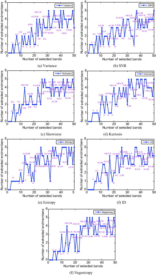
The Cuprite data in Figure 1.12(a) were used for endmember extraction where IN-FINDR was selected to extract the five mineral signatures, A, B, C, K, and M of major interest in the scene. Figure 21.8(a)–(g) plots extracted endmembers by IN-FINDR where seven BP criteria, variance, SNR, skewness, kurtosis, entropy, ID, and neg-entropy were used to prioritize bands to be used by PBDP. VD-estimated value for this scene was n_VD = 22 that was the same used for experiments in Chapter 20. Its twice value 2n_VD = 44 provided an upper bound used by PBDP. Therefore, the x-axis represents the number of prioritized bands used by PBDP starting from 0 to 50, and the y-axis is the number of extracted endmembers. When the number of extracted endmembers is less than 5, the extracted endmembers are specified by particular mineral signatures. As shown in Figure 21.8 the high-order statistics-based BP criteria generally performed better than second-order statistics-based BP criteria such as variance and SNR in the sense that fewer band numbers were required to extract five endmembers. The smallest and largest numbers of bands required to extract all the five mineral signatures were between 25 and 31. Compared to the results produced by PSDP in Figure 20.8, it is obvious that the number of spectral bands required by PBDP was greater than that by PSDP, which was between 18 and 28. This made sense because PSDP performed data compaction as opposed to PBDP, which essentially performed data reduction.

Figure 21.8 Endmember extraction results of PBDP prioritized cuprite scene using different BP criteria.

21.7.2 Land Cover/Use Classification

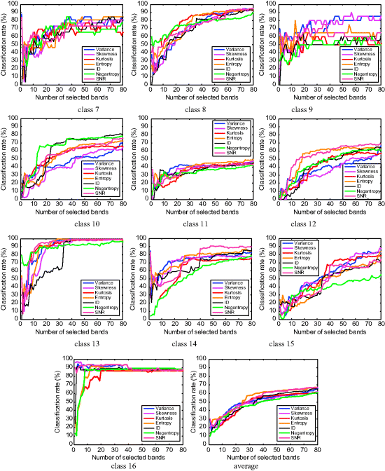
The Purdue Indiana Indian Pine Test Site in Figure 1.13 was also used for land cover/use classification. Figure 21.9 shows classification rates of MLC using PSDP based on seven BP criteria: variance colored by dark blue, SNR by light brown, skewness by purple, kurtosis by red, entropy by deep yellow, ID by black, and negentropy by green where the x-axis denotes the number of prioritized bands to be used to form image cubes for MLC classification, while the y-axis indicates MLC classification rates. In order to see how the number of bands affects the classification performance, the number of prioritized dimensions is run from 1 to the entire number of bands, 202.

Figure 21.9 MLC-classification rate of 16 classes versus the number of prioritized bands.

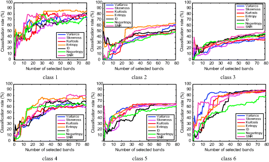
As shown in Figure 21.9, it is very clear that different classes required different number of spectral bands to achieve their best performance in classification. For instance, class 16 only required a few bands to achieve very high classification rate. Classes 1, 8, and 13 could also reach very high classification performance as long as went beyond 50. On the contrary, some of classes were very difficult to achieve such as high classification performance even if the entire 202 spectral bands were fully used. For example, classes 3 and 11 are considered as most difficult cases. This is probably due to the fact that the size of these two classes is too small or the ground truth information is not very accurate for these classes. As a consequence, the sample vectors in these two classes cannot provide reliable statistics to be used by MLC. From Figure 21.9 another interesting observation is worth noting where the classification of classes 7 and 9 started to slightly deteriorate when was greater than a certain number for some BP criteria. In particular, as the number of prioritized bands was increased the classification performance of these two classes was actually degraded. Other than these extreme cases we categorize classification performance into two groups. One is the cases that the classification rates never improved and saturated after a certain number of used prioritized bands, for example, classes 5, 13, and 16. Another is that the classification kept improving as the number of used prioritized bands was increased. It is particularly true for most of remaining classes, such as classes 1, 2, 3, 6, 8, 11, 12, and 15.

21.7.3 Linear Spectral Mixture Analysis

The 15-panel HYDICE images scene in Figure 1.15(a) and (b) was used to demonstrate the utility of PBDP in spectral unmxing. According to the ground truth in Figure 1.15(b) and (c) and four identified background signatures in Figure 1.17 there are at least nine signatures present in the scene that can be used to form a nine-signature matrix for a linear mixing model to perform spectral unmixing where FCLS was used to unmix all data sample vectors into their corresponding abundance fractions. Six BP criteria: variance, skewness, kurtosis, entropy, ID, and neg-entropy were used to evaluate the unmixing performance of PBDR and PBDE with the step size of band numbers set to one, that is, step size n_Δ = 1. Since VD provides a good estimate for a lower bound to n_initial for PBDE and an upper bound to n_final for PBDR, n_initial is set to n_VD = 9 for PBDE and 2n_VD = 18 for PBDR, respectively. From the scene there are five distinct panel signatures present in the field. If one band is required to accommodate one signature, it needs at least five bands to perform spectral unmixing in which case 5 provides a lower bound for n_initial = 9 used by PBDE. On the other hand, it has been shown in Chang (2003a, Chapter 5) and Heinz and Chang (2001) that 34 target signatures were sufficient for FCLS to work well in spectral unmxing. In this case, a sufficient number of bands to accommodate 34 target signatures was 34 that was used as an upper bound on n_final = 18 used by PBDR. Figure 21.10 plots six curves to represent the FCLS-unmixed abundance fractions of the 19 R pixels in the five rows in the range of [0,1] using the number of prioritized bands, ranging from 8 to 35, respectively, with the x-axis representing the number of prioritized bands to be used to form image cubes for FCLS versus y-axis indicating the FCLS-unmixed abundance fractions of 19 R panel pixels where six BP criteria: variance colored by dark blue-square, skewness by green-diamond, kurtosis by red-upside down triangle, entropy by cyan-open circle, ID by black-asterisk, and neg-entropy by purple-star were implemented. It is worth noting that when the number of bands, was smaller than 8, the results were fluctuated and not reliable as shown in the plots.

Figure 21.10 Plots of FCLS-unmixed abundance fractions versus number of prioritized bands for 19 red pixels in five row panels in HYDICE image by variance, skewness, kurtosis, entropy, ID, and negentropy.

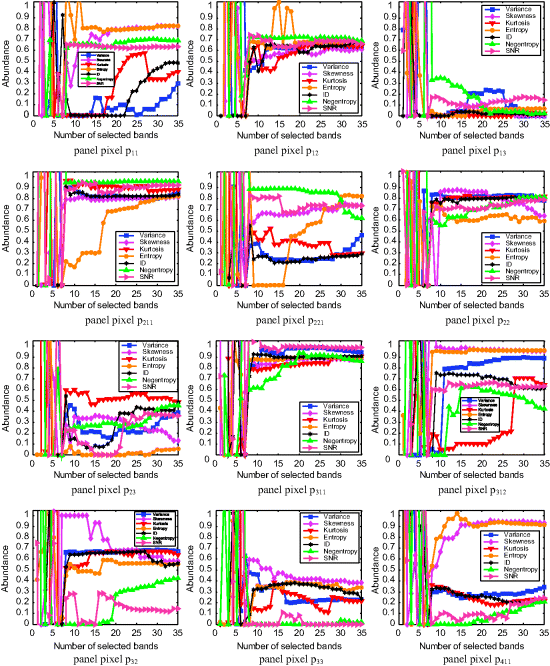
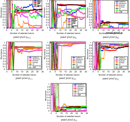
As shown in Figure 21.10, each panel pixel required a different value of to achieve its optimal performance in terms of its FCLS-unmixed abundance fraction compared to its true abundance in Figure 1.15(b). Since in the plot of the panel pixel p₅₂₁ the five curves by generated by variance (blue), skewness (green), kurtosis (red), ID (black), and negentropy (magenta) were identical, only two curves are shown in the plot, one for the five identical curves and the other for entropy (cyan). The quantification results in Figure 21.10 provided evidence that an optimal set of selected prioritized bands for one panel pixel was not necessarily also optimal for another panel pixel. For example, from visual inspection of the plots in Figure 21.10 the 19 panel pixels can be divided into three groups according to unmixing performance using various values of to select bands. The first group including panel pixels, p₁₂ (except entropy), p₂₁₁, p₂₂, p₃₁₁, p₄₃, p₅₁₁, p₅₂₁, p₅₂, p₅₃ required fairly stable values of to produce good FCLS-unmixed abundance fractions. The second group including panel pixels, p₁₃, p₃₂, p₃₃, p₄₁₁, p₄₂ needed moderately stable values of to produce good FCLS-unmixed abundance fractions. The third group including panel pixels, p₁₁, p₂₂₁, p₂₃, p₃₁₂, p₄₁₂ used fluctuated values of to produce good FCLS-unmixed abundance fractions. Interestingly, the three panel pixels p₁₁, p₁₂, and p₁₃ in row 1 happened to the case that covers all the three groups while all the four panel pixels, p₅₁₁, p₅₂₁, p₅₂, p₅₃ in row 5 falling in the same first group. Accordingly, using a fixed number of spectral bands to perform the conventional BS could not accomplish what PBDP could as demonstrated in Figure 21.10. However, a stopping rule for PBDP could be further determined by FCLS performance by comparing FCLS-unmixed results from using two consecutive band sets. Using the panel pixel p₅₁₁ as an example, PBDE would be terminated at = 8 if n_inital = 5 or 9 if n_inital = 9 when both results were very close. By contrast, PBDR would be terminated at = 18 if n_final = 18 or 35 if n_final = 35. So, choosing the values of n_inital and n_final was important. Nevertheless, the conducted experiments seemed to demonstrate that the range provided by VD, [n_VD,2n_VD] may not be optimal but indeed offered a feasible region for users by setting [n_initial,n_final] to [n_VD,2n_VD]. This issue will be further discussed in Chapter 22 by introducing a new concept of DDA.