22.5 Experiments for Dynamic Dimensionality Allocation

As demonstrated in PSDP and PBDP different signatures required various spectral dimensions/bands to effectively perform linear spectral unmixing due to their different spectral characteristics. These experiments provided evidence that a signature should have its own set of spectral dimensions/bands to characterize its spectral profile. In order for PSDP and PBDP to demonstrate progressive performance, three applications, endmember extraction, land cover/use classification, and spectral unmixing, were considered in Chapters 20 and 21 as the parameters, q and , varied ranging from n_VD to 2n_VD without knowing exactly what the values of q and were. DDA presented in Section 22.2 is developed to make an attempt of narrowing down the range of [n_VD,2n_VD] to best possible values that can be specified by DDA for dimensionality allocations for various signatures. In the following sections we calculate DDA for the three different image data sets which have been used for experiments conducted in Chapters 20 and 21 where the reference signatures were chosen to be the signature means of signatures of interest. Of course selection of an appropriate reference signature is also an interesting issue which will be discussed in Chapters 25, 27 and 28.

22.5.1 Reflectance Cuprite Data

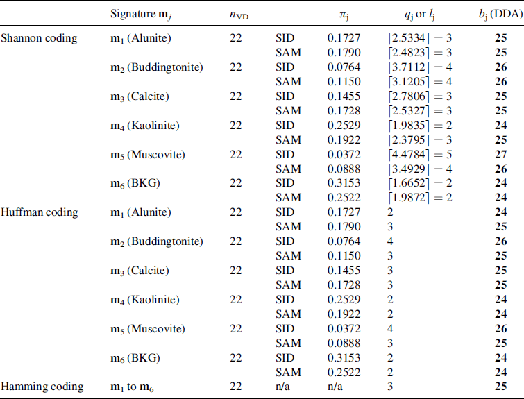
The reflectance Cuprite data in Figure 1.12 has been used for experiments in PART II to evaluate the effectiveness of an endmember extraction algorithm. According to the five known mineral signatures, m₁ = alunite, m₂ = buddingtonite, m₃ = calcite, m₄ = kaolinite, and m₅ = muscovite provided by the ground truth, DDA for these five signatures can be calculated by three coding methods, Shannon coding, Huffman coding, and Hamming coding and their results are tabulated in the last column of Table 22.1 where the signature discriminatory probabilities along with their corresponding lengths are calculated by two spectral measures, SAM and SID and provided in the table for reference. In addition, the value of VD, n_VD = 22 is also included in the table for comparison. As we can see from the table the values of DDA is in the range between 24 and 26.

Table 22.1 DDA results calculated by the three coding methods for reflectance cuprite data.

To substantiate the fact that the values provided by DDA are good estimates of q and IN-FINDR was used to extract endmembers. Table 22.2 tabulates extracted endmembers where SID was used to measure spectral similarity with a “1” indicating a success in extraction of one mineral signature and a “0” indicating a failure in missing extraction of one mineral signature.

Table 22.2 Endmember extraction using DDA for reflectance cuprite data.

An interesting finding in Table 22.2 is that using more bands did not guarantee better endmember extraction. For example, when bands were prioritized by skewness, IN-FINDR successfully extracted the mineral signature “B” if the value of was 22, but it failed at . Then it succeeded again when the value of was increased to 26. A similar phenomenon was also observed when bands were prioritized by variance to extract the mineral signature M where IN-FINDR was able to extract “M” when , but failed when . It then succeeded again when , but also failed again when . Also interesting is that n_VD = 22 turned out to be a very good estimate. On many occasions IN-FINDR successfully extracted mineral signatures at , but failed at , such as ID at , 25 failing to extract mineral signature “A,” entropy at failing to extract mineral signature “B”, variance at failing to extract mineral signature “C,” skewness at failing to extract mineral signature “K,” variance at , 26 failing to extract mineral signature “M.” Nevertheless, according to Table 22.2 the best result was the one using negentropy as a BP criterion to prioritize bands and DDA determined by Shannon coding or Huffman coding in which case all the five mineral signatures could be successfully extracted by IN-FINDR.

22.5.2 Purdue's Data

The Purdue Indiana Indian Pine test site in Figure 1.13 has been studied extensively in the literature for land cover/use classification. There are 16 classes of interest plus a background class. So, a total of 17 classes are present in the data. Each of 17 class signatures was found by the sample mean of 50% sample vectors randomly selected from its class and the other 50% will be used as test sample vectors for maximum likelihood classification (MLC). Table 22.3 tabulates DDA results using Shannon coding, Huffman coding, and Hamming coding where the signature discriminatory probabilities along with their corresponding lengths were calculated by two spectral measures, SAM and SID, and provided in the table for reference. In addition, the value of VD, n_VD = 29, was also included in the table for comparison.

Table 22.3 DDA results calculated by the three coding methods for the Purdue data.

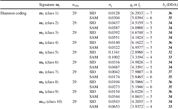
Table 22.4 tabulates the classification rates by MLC for 16 classes using DDA calculated in Table 22.3 where SID was used to measure spectral similarity. Also included in the table is the last column which gave the best classification rates with the optimal number of bands provided in parentheses.

Table 22.4 Classification rates of 16 classes in the Purdue data by MLC.

It is noted that in most cases MLC only needed a fewer prioritized bands to perform well without using all spectral bands, such as classes 7, 9, and 16 that did not require many spectral bands to produce the best results. There are some observations noteworthy. One is that second order statistic BPC generally performed better than high order and infinite order BPC due to the fact that the land covers of this particular scene are large, and the data samples are heavily mixed because of low spatial resolution and their contributions to statistics are mainly second-order statistics. This is not true for high-resolution hyperspectral data, such as HYDICE as will be demonstrated in the following section, which searches for rare data samples with pure signatures. On the other hand, it can be noted that in most cases using fewer band dimensions MLC could perform as well its using all dimensions. For instance, classes 7, 9, and 16 did not require more bands to produce the best results. There are only classes, 2, 3, 4, 6, 10, and 11 that required almost full dimensions to produce the best MLC results. Nevertheless, in general, DDA did provide some guidelines in selecting an appropriate value of for MLC to perform reasonably well. Finally, similar to endmember extraction Table 22.4 also demonstrates that using more bands did not necessarily produce better classification for each of seven used BP criteria (i.e., variance, SNR, skewness, kurtosis, entropy, ID, and negentropy), for example, classification of class 1 with SNR used as a BP criterion at versus 34 and 36 as well as with kurtosis used as a BP criterion at versus 58; classification of class 6 with skewness used as BP criterion at versus 34; classification of class 7 with variance used as BP criterion at and 37 versus 58 as well as with negentropy used as a BP criterion at versus 58; classification of class 16 with ID used as BP criterion at versus 58 as well as with entropy used as a BP criterion at versus 31. Nevertheless, according to Table 22.4, if DDA was used to determined the overall performance on MLC rates of 16 classes was generally improved over that produced by letting regardless of which BP criterion was used.

22.5.3 HYDICE Data

The five panel signatures in Figure 1.16 was used to unmix the 19 R panel pixels, p₁₁, p₁₂, p₁₃, p₂₁₁, p₂₂₁, p₂₂, p₂₃, p₃₁₁, p₃₁₂, p₃₂, p₃₃, p₄₁₁, p₄₁₂, p₄₂, p₄₃, p₅₁₁, p₅₂₁, p₅₂, p₅₃ in the HYDICE 15-panel scene in Figure 1.15 for abundance fraction quantification. According to the ground truth in Figures 1.15–1.17, nine signatures, m₁ = p₁, m₂ = p₂, m₃=p₃, m₄ = p₄, and m₅ = p₅ in Figure 1.16 and figure background signatures, m₆ = grass m₇ = road m₈ = tree and m₉ = interferer in Figure 1.17 were used as a desired set of signatures of interest. Table 22.5 tabulates DDA calculated by Shannon coding, Huffman coding, and Hamming coding using these nine signatures where SAM and SID were used to measure spectral similarity.

Table 22.5 DDA results calculated by the three coding methods for HYDICE data.

Table 22.6 tabulates FCLS-unmixed abundance fractions of the 19 R panel pixels with the number of selected prioritized spectral bands determined by n_VD and DDA using the three coding methods, and optimal number of bands to produce the best results in the last column.

Table 22.6 Unmixed abundance fractions of 19 panel pixels in the HYDICE data by FCLS.

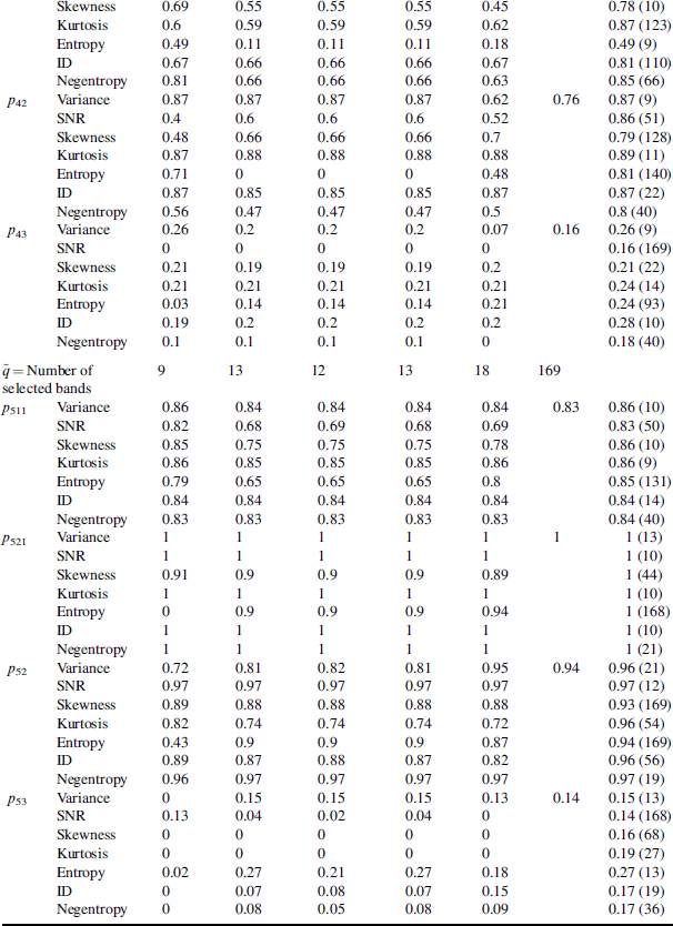
Several BP criteria were chosen to investigate DA. The results demonstrated that the skewness produced the best performance of FCLS abundance results because in most cases skewness criterion required less bands to achieve the optimal performance. On the other hand, for few panel pixels the best estimated p was around 9 that was the same as n_VD. For most of panel pixels p = 9 seemed to be insufficient but they still achieved good performance within p = 18 = 2 n_VD. Similar to AVIRIS data experiments conducted for endmember extraction in Section 22.5.1 and land cover/use classification in Section 22.5.2 the same conclusion that using more bands did not necessarily improve performance was also applied to HYDICE data. For example, when the three BP criteria, SNR, skewness and entropy were used to prioritize bands, the FCLS-unmixed abundance fraction of p₅₁₁ at was more accurate than that obtained at . Similarly, the same conclusions were also applied to the unmixed abundance fraction of the panel pixel p₂₁₁ with variance used as a BP criterion at against 13–15, 18; unmixed abundance fraction of the panel pixel p₂₂₁ with kurtosis used as a BP criterion at against 14–15, 18, FCLS-unmixed abundance fraction of the panel pixel p₄₁₂ with negentropy used as a BP criterion at versus 13–15,18; unmixed abundance fraction of the panel pixel p₁₂ with ID used as a BP criterion at against 13–15, 18. However, according to Table 22.6, if DDA was used to determine the overall performance on FCLS-unmixing 19 R panel pixels was generally better than that produced by letting regardless of which BP criterion was used.

Finally, several conclusions can be drawn from Tables 22.2, 22.4 and 22.6. First, a BP criterion has a significant impact on performance. Its selection must be determined by a specific application. Second, it is generally not true that using more BP-ranked bands will yield better performance. This may be due to the fact that high prioritized bands will also be highly correlated. As a result, redundant bands are also very likely selected and may not provide any benefit but rather conflicting information. This issue can be resolved by band de-correlation (BD) to be discussed in Chapter 23. Last but not least, as shown in Chapter 20, VD can appropriately estimate the number of dimensions to be retained after dimensionality reduction, q. But when it comes to band selection, VD seems to under-estimate the value of . In this case, DDA provides a better estimate of .