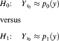
3.2 Neyman–Pearson Detection Problem Formulation

In Section 2.2.1 a binary hypothesis testing problem (2.1) is used to formulate the pure-sample target detection as two hypotheses, H₀ and H₁, which represent the absence and presence of a signal source in an observed sample r, respectively. This section places its main focus on a particular type of detection problem when there is no prior knowledge of the two hypotheses and cost functions. It is generally called the Neyman–Pearson detection problem cast by (2.9–2.11).

More specifically, assume that the observation process is described by a random process Y_t. When this process is observed at a particular time instant t = t₀, it is referred to as an observation y which can be described by a random variable . If the probability distribution of is further assumed to be P(y) with its probability density function given by p(y), the binary hypothesis testing problem (2.1) can be described by

(3.1)

where the hypotheses H₀ and H₁ can be observed from the variable whose probability distributions are derived from p(y) under each hypothesis, denoted by p₀(y) under H₀ and p₁(y) under H₁. The hypotheses “H₀” and “H₁” are generally called “null hypothesis” and “alternative hypothesis,” respectively. In applications of signal processing and communications, “H₁,” such as in Section 2.2.1, represents the case when the signal is present along with noise, while the hypothesis “H₀” indicates that no signal is present. So, when hypothesis “H₁” is true, it implies that there is a signal present in the observation y.

Assume that the observation y is the data sample vector denoted by r and the observation space Γ is denoted by data sample vector space. Using (2.2) and Figure 2.1 and renumbering (2.9)–(2.11), P_D(δ) is defined as the detection probability/rate or detection power specified by (2.10),

(3.2)

and P_F(δ) as the false alarm probability/rate specified by (2.9),

(3.3)

An NP detector, denoted by δ^NP(r), is obtained by solving the following constrained optimization problem specified by (2.11) and recapped as follows:

(3.4)

where β is prescribed and known as the significant level of test and the maximum is sought over all possible decision rules, δ(r). The well-known Neyman–Pearson lemma shows that the optimum solution to (3.4) turns out to be a likelihood ratio test, Λ(r), similar to (2.8) and given by

(3.5)

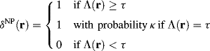
where Λ(r) = p₀(r)/p₁(r), the threshold τ is determined by the constraint β, and γ is the probability of saying H₁ when Λ(r) = τ. By virtue of δ^NP(r), P_D and P_F in (3.2)–(3.3) can be obtained and expressed as follows:

(3.6)

(3.7)

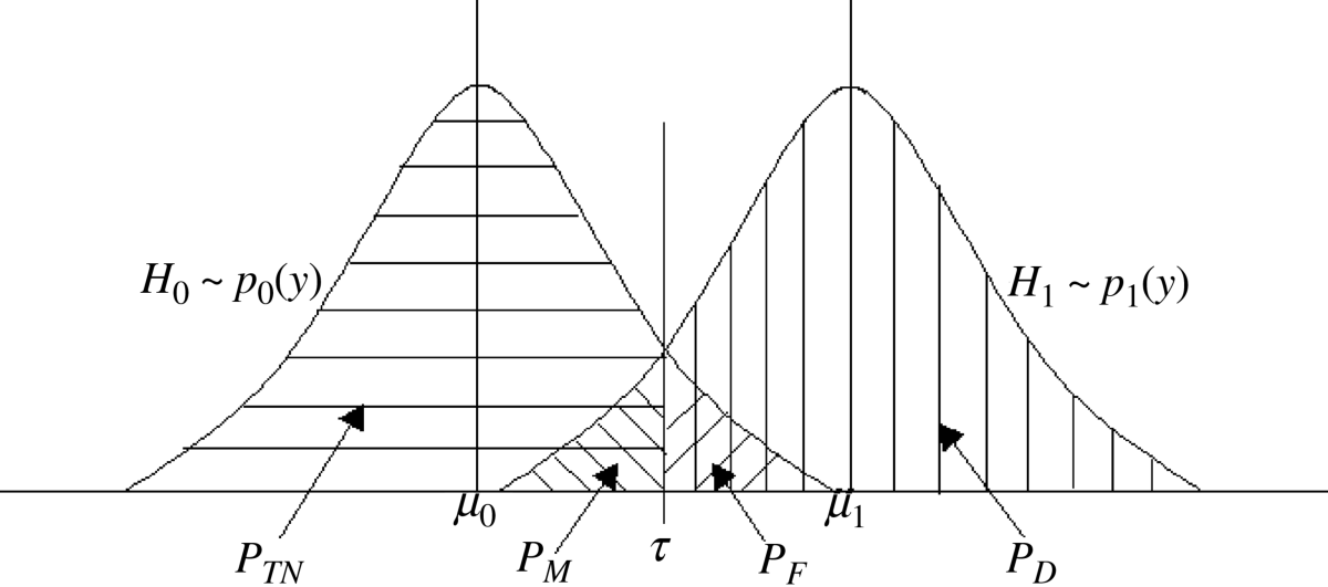
with τ determined by P_F = β via (3.3). Details of signal detection theory can be found in Poor (1994). Figure 3.1 shows how a decision can be made by adjusting threshold τ using (3.6) and (3.7) where the regions corresponding to four decisions described in Section 3.1 P_M = 1 − P_D (decision 1), P_D (decision 2), P_F (decision 3), and P_TN = 1 − P_F (decision 4) are indicated with different shaded areas.

Figure 3.1 An illustration of probabilities P_D, P_F, P_M, and P_TN.

A final remark is noteworthy. According to standard detection theory four types of decisions described in Section 3.1 can be made based on the binary hypothesis testing problem specified by (3.1). However, in some applications there is a fifth decision that is no action to be taken due to insufficient knowledge. For example, in automatic target recognition (Parker et al., 2005a, 2005b; Blasch et al., 1999; Blasch and Broussard, 2000; Bauman et al., 2005), documentation analysis such as character recognition (Suen et al., 1980) and text detection in video images (Du et al., 2003), and biometric recognition (Du and Chang, 2008), when the level of confidence of making a decision is low due to the lack of knowledge, an alternative option is rejection. However, this approach can be actually interpreted in the context of what is the so-called randomized decision in statistical detection theory. When the detector statistics, Λ(r) specified by (3.5), is equal to the threshold τ, two actions can be taken. One is doing nothing but rejection which is the fifth type of decision as described above in addition to the four described in Section 3.1. The other is to force the detector to make a soft decision on two hypotheses to express the confidence level of each decision in terms of its probability. As a consequence, such a random decision is better off than a rejection since the latter simply does not make any decision by rejecting.