
13.2. Reliability
Reliability is the degree to which multiple measurements on asubject agree. Typically this includes establishing appropriate levels of inter-rater reliability, test-retest reliability, and internal consistency. Inter-rater reliability is an assessment of the agreement between different raters' scores for the same subject at the same point in time. Test-retest reliability summarizes the consistency between different measurements on the same subject over time. Intra-rater reliability is a special case of test-retest reliability where measurements are obtained by the same rater over time on the same subject. Internal consistency evaluates the consistency with the items of a scale assessing the same construct. In thissection we discuss several approaches to quantitatively assessing reliability and provide numerical examples using SAS.
13.2.1. Inter-Rater Reliability
A measure is said to have inter-rater reliability if ratings by different individuals at the same time on the same subject are similar. Inter-rater reliability is not only assessed when validating a newly created instrument, but is also used to prior to beginning a clinical trial to quantify the reliability of the measure as used by the raters participating in the trial. In the latter case, these evaluation sessions are used to both train and quantify inter-rater reliability, even when a scale with established reliability is being used.
13.2.2. Kappa statistic
The Kappa statistic (κ) is the most commonly used tool for quantifying the agreement between raters when using a dichotomous or nominal scale, while the intraclass correlation coefficient (ICC) or concordance correlation coefficient (CCC) are the recommended statistics for continuous measures. The use of κ will be discussed in this section while examples of the use of ICC and CCC are presented later (see Sections 13.2.5 and 13.2.7).
The κ statistic is the degree of agreement above and beyond chance agreementnormalized by the degree of attainable agreement above what would be predicted by chance. This measure is superior to simple percent agreement as it accounts for chance agreement. For instance, if two raters diagnose a set of 100 patients for the presence or absence of a rare disease, they would have a high percentage of agreement even if they each randomly chose one subject to classify as having the disease and classified all others asnot having the disease. However, the high agreement would likely not result in a high value for κ.
| Rater 1 | Rater B | Total | |
|---|---|---|---|
| Yes | No | ||
| Yes | n11 | n12 | n1. |
| No | n21 | n22 | n2. |
| Total | n.1 | n.2 | n |
To define κ, consider the notation for a 2 × 2 table displayed in Table 13.1 and let pij = nij/n, pi. = ni./n and p.j = n.j/n. The value of κ can be estimated by using the observed cell proportions as follows:
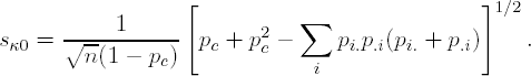
where pa is given by pa = Σi pii and represents the observed proportion of agreement in these data. Further,pc is defined as pc = Σi pi.p.i and represents the proportion of agreement expected by chance. Confidence intervals can be computed using the asymptotic standard deviation of κ provided by Fleiss et al (1969):

where

Fleiss (1981) provided the variance of κ under the null hypothesis (κ = 0) which can be used to construct a large sample test statistic:
For exact inference calculations, the observed results are compared with the set of all possible tables with the same marginal row and column scores. See Agresti (1992) or Mehta and Patel (1983) for details on computing exact tests for contingency table data.
EXAMPLE: Schizophrenia diagnosis example
The simplest example of inter-rater reliability study is when two raters rate a group of subjects as to whether certain criteria (e.g., diagnosis) are met using a diagnostic instrument. The κ statistic is the traditional approach to assessing interrater reliability in such circumstances. PROC FREQ provides for easy computation of the κ statistic, with inferences based on either large sample assumptions or an exact test.
Bartko (1976) provided an example where two raters classified subjects as to whether they had a diagnosis of schizophrenia. These data, modified for this example, are displayed in Table 13.2 and will be used to demonstrate the computation of the κ statistic in SAS.
| Rater A | Rater B | |
|---|---|---|
| Yes | No | |
| Yes | 5 | 3 |
| No | 1 | 21 |
Program 13.1 uese the FREQ procedure to compute the κ statistic in the schizophrenia diagnosis example.
Example 13-1. Computation of the κ statistic
data schiz;
    input rater_a; rater_b; num;
    cards;
    yes yes  5
    yes no   3
    no  yes  1
    no  no  21
    ;
proc freq data=schiz;
    weight num;
    tables rater_a*rater_b;
    exact agree;
run; |
Example. Output from Program 13.1
Simple Kappa Coefficient

                   Kappa (K)                 0.6296
                   ASE                       0.1665
                   95% Lower Conf Limit      0.3033
                   95% Upper Conf Limit      0.9559
Test of H0: Kappa = 0
ASE under H0 0.1794
Z 3.5093
One-sided Pr > Z 0.0002
Two-sided Pr > |Z| 0.0004
Exact Test
One-sided Pr >= K 0.0021
Two-sided Pr >= |K| 0.0021
Sample Size = 30 |
Note that in this example the observed agreement is p11 + p22 = 26/30 = 86.7%. However, a 64% agreement can be expected by chance given the observed marginals, i.e.,

Output 13.1 shows that the estimated κ is 0.6296 with a 95% confidence interval of (0.3033,0.9559). This level of agreement (in the range of 0.4 to 0.8) is considered moderate, while κ values of 0.80 and higher indicate excellent agreement (Stokes et al, 2000). Output 13.1 also provides for testing the null hypothesis of κ =0.By including the EXACT AGREE statement in Program 13.1, we obtained both large sample and exact inferences. Both tests indicate the observed agreement is greater than chance (p = 0.0004 using the z-statistic and p = 0.0021 using the exact test).
Two extensions of the κ measure of agreement, the weighted κ and stratified κ, are also easily estimated using PROC FREQ. A weighted κ is applied to tables larger than 2 by 2 and allows different weight values to be placed on different levels of disagreement. For example, on a 3-point scale, i.e., (0,1,2), a weighted κ would penalize cases where the raters differed by 2 points more than cases where the difference was one. Both Cicchetti and Allison (1971) and Fleiss and Cohen (1973) havepublished weight values for use in computing a κ statistic. Stokes et al (2000) provides an example of using SAS to compute a weighted κ statistic.
When reliability is to be assessed across several strata, a weighted average of strata specific κ's can be produced. SAS uses the inverse variance weighting scheme,see PROC FREQ documentation for details.
The κ statistic has been criticized because it is a function of not only thesensitivity (proportion of cases identified or true positive rate) and specificity (proportion of non-cases correctly identified) of an instrument, but also of the overall prevalence of cases (base rate). For instance, Grove et al.(1981) pointed out that with sensitivity and specificity held constant at 0.95, a change in the prevalence can greatly influence the value of κ. Spitznagel and Helzer (1985) noted that a diagnostic procedure showing a high κ in a clinical trial with a high prevalence will have a lowervalue of κ in a population based study, even when the sensitivity and specificity are the same. Thus, comparisons of agreement across different studies where the base rate (prevalence) differs is problematic with the κ statistic.
13.2.3. Proportion of Positive Agreement and Proportion of Negative Agreement
One approach to overcoming this drawback with the κ statistic is to use a pair of statistics: the proportion of positive agreement, p+, and the proportion of negative agreement, p–. Consider the situation where two raters classify a set of patients as having or not having a specific disease. The first measure, p+, is the conditional probability that a rater will give a positive diagnosis given that the other rater has given a positive diagnosis. Similarly, p– is the conditional probability that a rater will give a negative diagnosis given that the other rater has given a negative diagnosis. These conditional probabilities are defined as follows
and are analogous to characterizing a diagnostic tests sensitivity (the proportionof patients with a disease correctly identified) and specificity (the proportion of patients without the disease correctly identified). Note that p+ can be viewed as a weighted average of the sensitivities computed considering each rater as the gold standard separately and p– can be viewed as a weighted average of the specificities computed considering each rater as the gold standard separately. In addition, sensitivity and specificity are not even applicable in situations where there is no gold standard test. However, p+ and p– are still useful statistics in such situations, e.g., p+ is the conditional probability that a rater will give a positive diagnosis given that theother rater has given a positive diagnosis.
Program 13.2 demonstrates how to compute p+, p– and associated confidence intervals in the schizophrenia diagnosis example. The confidence intervals are computed using formulas based on the delta method provided by Graham and Bull (1998).
Example 13-2. Computation of the proportion of positive agreement, proportion of negative agreement and associated confidence intervals
data agreement;
    set schiz nobs=m;
    format p_pos p_neg lower_p lower_n upper_p upper_n 5.3;
    if rater_a='yes' and rater_b='yes' then d=num;
    if rater_a='yes' and rater_b='no'  then c=num;
    if rater_a='no'  and rater_b='yes' then b=num;
    if rater_a='no'  and rater_b='no'  then a=num;
    n=a+b+c+d;
    p1=a/n; p2=b/n; p3=c/n; p4=d/n;
    p_pos=2*d/(2*d+b+c);
    p_neg=2*a/(2*a+b+c);
    phi1=(2/(2*p4+p2+p3))-(4*p4/((2*p4+p2+p3)**2));
    phi2_3=-2*p4/(((2*p4+p2+p3)**2));
    gam2_3=-2*p1/(((2*p1+p2+p3)**2));
    gam4=(2/(2*p1+p2+p3))-(4*p1/((2*p1+p2+p3)**2));
    sum1=(phi1*p4+phi2_3*(p2+p3))**2;
    sum2=(gam4*p1+gam2_3*(p2+p3))**2;
    var_pos=(1/n)*(p4*phi1*phi1+(p2+p3)*phi2_3*phi2_3-4*sum1);
    var_neg=(1/n)*(p1*gam4*gam4+(p2+p3)*gam2_3*gam2_3-4*sum2);
    lower_p=p_pos-1.96*sqrt(var_pos);
    lower_n=p_neg-1.96*sqrt(var_neg);
    upper_p=p_pos+1.96*sqrt(var_pos);
    upper_n=p_neg+1.96*sqrt(var_neg);
    retain a b c d;
    label p_pos='Proportion of positive agreement'
          p_neg='Proportion of negative agreement'
          lower_p='Lower 95% confidence limit'
          lower_n='Lower 95% confidence limit'
          upper_p='Upper 95% confidence limit'
          upper_n='Upper 95% confidence limit';
    if _n_=m;
proc print data=agreement noobs label;
var p_pos lower_p upper_p;
proc print data=agreement noobs label;
var p_neg lower_n upper_n;
run; |
Example. Output from Program 13.2
Proportion     Lower 95%     Upper 95%
               of positive    confidence    confidence
                agreement       limit         limit

                  0.714         0.446         0.983

               Proportion     Lower 95%     Upper 95%
               of negative    confidence    confidence
                agreement       limit         limit

0.913 0.828 0.998 |
It follows from Output 13.2 that in the schizophrenia diagnosis example we observed 71.4% agreement on positive ratings and 91.3% agreement on negative ratings. Using the Graham-Bull approach with these data, we compute the following 95% confidence intervals: (0.446, 0.983) for agreement on positive ratings, and (0.828, 0.998) for agreement on negative ratings.
13.2.4. Inter-Rater Reliability: Multiple Raters
Fleiss (1971) proposed a generalized κ statistic for situations with multiple (more than two) raters for a group of subjects. It follows the form of κ above, where percent agreement is now the probability that a randomly chosen pair of raters will give the same diagnosis or rating.
EXAMPLE: Psychiatric diagnosis example
Sandifer et al. (1968) provided data from a study in which 6 psychiatrists provided diagnoses for each of 30 subjects. Subjects were diagnosed with either depression, personality disorder, schizophrenia, neurosis, or classified as not meeting any of the diagnoses.
Program 13.3 computes the expected agreement (pc), percent agreement (pa), kappa statistic (κ) and a large sample test statistic for testing the null hypothesis of no agreement beyond chance in the psychiatric diagnosis example. These statistics were calculated using the formulas provided by Fleiss (1971):

where N is the total number of subjects, r is the number of raters and the subscripts i and j refer to the subject and diagnostic category, respectively.
Example 13-3. Computation of agreement measures
data diagnosis;
    input patient depr pers schz neur othr @@;
    datalines;
1  0 0 0 6 0 2  0 3 0 0 3 3  0 1 4 0 1 4  0 0 0 0 6 5  0 3 0 3 0
6  2 0 4 0 0 7  0 0 4 0 2 8  2 0 3 1 0 9  2 0 0 4 0 10 0 0 0 0 6
11 1 0 0 5 0 12 1 1 0 4 0 13 0 3 3 0 0 14 1 0 0 5 0 15 0 2 0 3 1
16 0 0 5 0 1 17 3 0 0 1 2 18 5 1 0 0 0 19 0 2 0 4 0 20 1 0 2 0 3
21 0 0 0 0 6 22 0 1 0 5 0 23 0 2 0 1 3 24 2 0 0 4 0 25 1 0 0 4 1
26 0 5 0 1 0 27 4 0 0 0 2 28 0 2 0 4 0 29 1 0 5 0 0 30 0 0 0 0 6
;
%let nr=6; * Number of raters;
data agreement;
    set diagnosis nobs=m;
    format pa pc kappa kappa_lower kappa_upper 5.3;
    sm=depr+pers+schz+neur+othr;
    sum0+depr; sum1+pers; sum2+schz; sum3+neur; sum4+othr;
    pi=((depr**2)+(pers**2)+(schz**2)+(neur**2)+(othr**2)-sm)/(sm*(sm-1));
    tot+((depr**2)+(pers**2)+(schz**2)+(neur**2)+(othr**2));
    smtot+sm;
    if _n_=m then do;
        avgsum=smtot/m;
        n=sum0+sum1+sum2+sum3+sum4;
        pdepr=sum0/n; ppers=sum1/n; pschz=sum2/n; pneur=sum3/n; pothr=sum4/n;
        * Percent agreement;
        pa=(tot-(m*avgsum))/(m*avgsum*(avgsum-1));
        * Expected agreement;
        pc=(pdepr**2)+(ppers**2)+(pschz**2)+(pneur**2)+(pothr**2);
        pc3=(pdepr**3)+(ppers**3)+(pschz**3)+(pneur**3)+(pothr**3);
        * Kappa statistic;
        kappa=(pa-pc)/(1-pc);
    end;
    * Variance of the kappa statistic;
    kappa_var=(2/(n*&nr*(&nr-1)))*(pc-(2*&nr-3)*(pc**2)+2*(&nr-2)*pc3)/((1-pc)**2);
    * 95% confidence limits for the kappa statistic;
    kappa_lower=kappa-1.96*sqrt(kappa_var);
    kappa_upper=kappa+1.96*sqrt(kappa_var);
    label pa='Percent agreement'
          pc='Expected agreement'
          kappa='Kappa'
          kappa_lower='Lower 95% confidence limit'
          kappa_upper='Upper 95% confidence limit';
    if _n_=m;
proc print data=agreement noobs label;
    var pa pc;
proc print data=agreement noobs label;
    var kappa kappa_lower kappa_upper;
run; |
Example. Output from Program 13.3
Percent     Expected
                        agreement    agreement

                          0.556        0.220

                           Lower 95%     Upper 95%
                           confidence    confidence
                  Kappa      limit         limit

0.430 0.408 0.452 |
Output 13.3 lists the percent agreement (pa = 0.556), expected agreement (pc = 0.22) and kappa (κ = 0.43). It also shows the 95% confidence limits for κ. The lower limit is well above 0 and thus there is strong evidence that agreement in the psychiatric diagnosis example is in excess of chance. As there is evidence for agreement beyond chance, as a follow-up analysis one may be interested in assessing agreement for specific diagnoses. Fleiss (1971) describes such analyses—computing the conditional probability that a randomly selected rater assigns a patient with diagnosis j given a first randomly selected rater chose diagnosis j. This is analogous to the use of p+ describedin the previous section.
13.2.5. Inter-Rater Reliability: Rating Scale Data
The inter-rater rel iability of a rating scale is a measure of the consistency of ratings from different raters at the same point in time. The intra-class correlation coefficient (ICC) or the concordance correlation coefficient (CCC) arethe recommended statistics for quantifying inter-rater reliability when using continuousmeasures. Shrout et al. (1979) presented multiple forms of the ICC along with discussions of when to use various forms. Here we present the statistics for estimating ICCs from a two-way ANOVA model:
- Model outcome = Subjects + Raters.
We will consider the case when randomly selected raters rate each subject (ICC1) and also the case when the selected raters are the only ones of interest (ICC2). ICC1 maybe of interest when it can be assumed the raters in a study represent a random sample ofa population for which the researchers would like to generalize to. ICC2 may be used in rater training sessions prior to a clinical trial with pre-selected raters. The two coefficients are defined as follows:
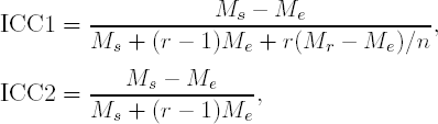
where r is the number of raters, n is the number of subjects and Ms, Mr, and Me are the mean squares for subjects, raters, and error, respectively.
Shrout et al. (1979) also provides formulas for estimating the variances for each form of the ICC and a discussion of a one-way ICC when different sets of raters score each subject. The null hypothesis of a zero ICC can be tested with an F-test given by F = Ms/Me with (n – 1) and (r – 1)(n – 1) degrees of freedom. As the ICC statistic and the associated tests and confidence intervals are based on summary statistics produced in a typical ANOVA, these can be easily computed using either the GLM or MIXED procedure. The SAS library of sample programs provides a macro that computes all versions of the ICC per Shrout's formulas as well as others:
Further discussion of the ICC and related statistics is provided later in Section 13.2.7.
EXAMPLE: Rater training session example
We will now describe an example of a rater training session performed at the beginning of a clinical trial. While in the previous examples a small number of raters assessed many subjects, in this example many raters assess only a small number of subjects (often 1 or 2). This situation is more commonplace in clinical trials. a rater training session is a good example of this setting.
Prior to implementing an antidepressant clinical trial, Demitrack et al. (1998) assessed the inter-rater reliability of 85 raters for the Hamilton Rating Scale for Depression (HAMD)(Hamilton, 1960) as part of a rater training session. The HAMD total score isa measure of the severity of a patient's depression with higher scores indicating more severe depression. The main goal of the session was to establish consistency in the administration and interpretation of the scale across multiple investigational sites. From a statistical perspective, the goals were to reduce variability (and thus increase power) by training raters to score using the scale in a similar fashion and to identify potential outlier raters prior to the study.
Raters independently scored the HAMD from a videotaped interview of a depressed patient. Fleiss' generalized κ, as described in the previous section, was used to summarize the inter-rater reliability for this group of raters. As only one subject was assessed, agreement was computed across items of a scale rather than across subjects. The percent agreement now represents the probability that two randomly selected raters provided the same rating score for a randomly selected item. The observed agreement and κ for these data are 0.55 and 0.4.
While an overall summary of agreement provides information about the scale and raters, it is also of importance in a multi-site clinical trial to identify raters who are outliers. These raters have the potential to increase variability in the outcome variable and thus reduce the power to detect treatment differences. Using the mode of the groupof raters as the gold standard, Demitrack et al (1998) computed the percent agreement and inter-class correlation coefficient for each rater (relative to the gold standard). Rater ICCs ranged from 0.40 to 1.0, with only two raters scoring below 0.70. Percentage agreement was also assessed by item in order to identity areas of disagreement for follow-up discussion.
Rater training sessions followed the discussion of the initial videotape results and the session concluded with raters scoring a videotape of the same patient in an improved condition. Demitrack et al concluded that the training did not clearly improve the agreement of the group, though they were able to use the summary agreement statistics to identify raters who did not score the HAMD consistent with the remainder of the group prior to implementing the trial. While Demitrack et al. used percent agreement and ICC in their work, the average squared deviation (from the gold standard) is another statistic that has been proposed for use in summarizing inter-rater reliability data (Channon and Butler, 1998).
13.2.6. Internal consistency
Measures of internal consistency assess the degree to which each item of a rating scale measures the same construct. Cronbach's α, a measure of the average correlation of items within a scale, is a commonly used statistic to assess internal consistency(Cronbach, 1951):
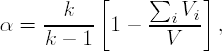
where k is the number of items, Vi is the variance of the ith item and V is the variance of the total score.
Cronbach's α ranges from 0 to 1, with higher scores suggesting good internal consistency. It is considered to be a lower bound of the scale's reliability (Shrout, 1998). Perrin suggested 0.7 as a minimal standard for internal consistency when making group comparisons, with a higher standard of at least 0.90 when individual comparisons areto be used (Perrin et al, 1997). Cronbach's α is a function of the average inter-item correlation and the number of items. It increases as the number of related items in the scale increases. If α is very low, the scale is either too short or the items have very little in common (delete items which do not correlate with the others). On theother hand, extremely high scores may indicate some redundancy in the rating scale. Cronbach's α; can be computed using the CORR procedure.
EXAMPLE: EESC rating scale example
Kratochvil et al. (2004) reported on the development of a new rating scale with 29items to quantify expression and emotion in children (EESC). Data from an interim analysis of a validation study involving 99 parents of children with attention-deficit hyperactivity disorder are used here to illustrate the assessment of internal consistency.
Program 13.4 utilizes PROC CORR for computing internal consistency and item-to-total correlations in the EESC rating scale example. The EESC data set used in the program can be found on the book's web site.
Example 13-4. Computation of Cronbach's α;
proc corr data=eesc alpha;
    var eesc1 eesc2 eesc3 eesc4 eesc5 eesc6 eesc7 eesc8 eesc9 eesc10
        eesc11 eesc12 eesc13 eesc14 eesc15 eesc16 eesc17 eesc18 eesc19 eesc20
        eesc21 eesc22 eesc23 eesc24 eesc25 eesc26 eesc27 eesc28 eesc29;
run; |
Example. Output from Program 13.4
Cronbach Coefficient Alpha

                     Variables              Alpha

                     Raw                 0.900146
                     Standardized        0.906284

           Cronbach Coefficient Alpha with Deleted Variable

                   Raw Variables             Standardized Variables

 Deleted     Correlation                   Correlation
 Variable     with Total          Alpha     with Total          Alpha

 EESC1          0.291580       0.899585       0.281775       0.906622
 EESC2          0.545988       0.895571       0.564959       0.901673
 EESC3          0.591867       0.894167       0.593887       0.901158
 EESC4          0.672391       0.892861       0.672410       0.899748
 EESC5          0.247457       0.901908       0.240618       0.907326
 EESC6          0.458779       0.896995       0.448555       0.903730
 EESC7          0.478879       0.896641       0.472999       0.903300
EESC8 0.665566 0.893793 0.675876 0.899685 EESC9 0.505510 0.896072 0.498409 0.902853 EESC10 0.651696 0.894064 0.652332 0.900110 EESC11 0.666862 0.893457 0.677098 0.899663 EESC12 0.380065 0.898422 0.395765 0.904652 EESC13 0.368793 0.898586 0.363621 0.905211 EESC14 0.623236 0.893495 0.614713 0.900785 EESC15 0.392515 0.898165 0.407936 0.904440 EESC16 0.389488 0.898200 0.396298 0.904643 EESC17 0.624384 0.894600 0.637290 0.900380 EESC18 0.485442 0.896484 0.480872 0.903162 EESC19 -.015219 0.907669 -.000957 0.911384 EESC20 0.707713 0.891929 0.710875 0.899052 EESC21 0.550139 0.895331 0.540735 0.902104 EESC22 0.639571 0.894357 0.649545 0.900160 EESC23 0.436383 0.897693 0.435663 0.903956 EESC24 0.423187 0.897806 0.424149 0.904157 EESC25 0.294496 0.901074 0.292439 0.906439 EESC26 0.313600 0.899842 0.315250 0.906047 EESC27 0.514513 0.896137 0.512612 0.902602 EESC28 0.362475 0.898664 0.367987 0.905135 EESC29 0.509206 0.896090 0.508525 0.902674 |
Output 13.4 provides estimates of Cronbach's α using both raw data and with items standardized to have a standard deviation of 1.0. The standardized scores may be useful when there are large differences in item variances. The results indicate an acceptable level of internal consistency (α > 0.90).
The output also lists the correlation of each item to the remaining total score, as the value of Cronbach's α with each individual item deleted from the scale, as well as the correlation of each item score with the remaining total score. The item-to-total correlations were at least moderate for all items except number 19. The low item-to-total for item 19 led to further investigation. It was found that the item ("My child shows a range of emotions") was being interpreted in both a positive and negative manner by different parents, leading to the poor correlation. Thus, this item was removed in theremoved version of the scale.
Despite the acceptable properties, it may still be of interest to consider a more concise scale, one that would be less burdensome on the respondent. From Output 13.3, the removal of any single item would not bring about a substantial change in Cronbach's α . Inter-item correlations (also produced by Program 13.3 but not included in the output to save space) could be examined to make scale improvements in this situation.
The PROC CORR documentation contains another example of the computation of Cronbach's α.
13.2.7. Test-Retest Reliability
Test-retest reliability indicates the stability of ratings on the same individual at two different times while in the same condition. For test-retest assessments, the re-test ratings should be taken long enough after the original assessment to avoid recall bias and soon enough to limit the possibility of changes in the condition of the subject. For continuous measures, Pearson's correlation coefficient is often used to quantify the relationship between two measures. However, as this only captures correlation between measures and not whether the measures are systematically different, the ICC or CCC are preferred measures for quantifying test-retest reliability. For instance, if the second (re-test) measurement is always 2 points higher than the first, Pearson's correlation coefficient will be 1 while the ICC and CCC will be reduced due to the systematic differences. Considering these data as a scatterplot with the x and y axis representing the first and second measurements on the subjects, Pearson's correlation coefficient assesses deviations from the best fitting regression line. The CCC is a measure that assesses departures from the line of identity (a 45 degree line). Thus, systematic departures will reduce the CCC. The closely related ICC statistic is the proportion of the total variability in scores that is due tothe variability among subjects. Thus, an ICC close to 1 indicates that little of the variability in scores is due to rater differences and thus the test-retest reliability is excellent.
The (2-way) ICC and CCC statistics are given by (Shrout and Fleiss, 1979; Lin et al, 2002)

where Ms and Me are the mean squares for subjects and error, respectively, r is Pearson's correlation coefficient between observations at the first and second time points, i.e., Yi1 and Yi2, and s12 and s22 are the sample variances of the outcomes at the first and second time points. The 95% confidence limits for ICC are given below
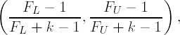
where k is the number of occasions,

and F0 = Ms/Me.
Lin (1989) demonstrated that
is asymptotically normal with mean
and variance
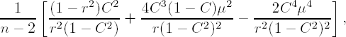
where C is the true concordance correlation coefficient, r is Pearson's correlation coefficient defined above and μ =(μ1 − μ2)/√σ1σ2. Confidence intervals can be formed by replacing the parameters with their estimates.
An alternative testing approach to assessing inter-rater reliability is provided by the Bradley-Blackwood test. This approach simultaneously tests the null hypothesis of equal means and variances at the first and second assessments (Sanchez and Binkowitz 1999). The Bradley-Blackwood test statistic B, which has an F distribution with 2 and n – 2 degrees of freedom, is as follows:
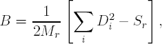
where Di = Yi1 – Yi2, and Sr and Mr are the error sum of squares and mean square error of the regression of Di on Ai = (Yi1 + Yi2)/2.
EXAMPLE: Sickness inventory profile example
Deyo (1991) provided data on the sickness inventory profile (SIP) from a clinical trial for chronic lower back pain. Data were obtained from 34 patients deemed unchanged in severity with measures taken two weeks apart.
Program 13.5 computes the ICC and associated large sample 95% confidence limits. As the ICC is computed from mean squares in an ANOVA model, it is easily computable using output from the PROC MIXED procedure as demonstrated below.
Example 13-5. Computation of the ICC, CCC and Bradley-Blackwood test
options ls=70;
data inventory;
    input patient time sip @@;
    datalines;
1 1  9.5  9 1  7.3 17 1  4.0 25 1 10.1 33 1  4.6
1 2 12.3  9 2  6.1 17 2  3.6 25 2 15.7 33 2  4.3
2 1  3.6 10 1  0.5 18 1  6.6 26 1 10.2 34 1  4.6
2 2  0.4 10 2  1.0 18 2  7.0 26 2 15.2 34 2  4.3
3 1 17.4 11 1  6.0 19 1 13.8 27 1  9.5
3 2  7.4 11 2  3.1 19 2 10.1 27 2  8.2
4 1  3.3 12 1 31.6 20 1  9.8 28 1 19.1
4 2  2.2 12 2 16.6 20 2  8.3 28 2 21.9
5 1 13.4 13 1    0 21 1  4.8 29 1  5.6
5 2  6.0 13 2  2.3 21 2  2.9 29 2 10.6
6 1  4.1 14 1 25.0 22 1  0.9 30 1 10.7
6 2  3.5 14 2 12.2 22 2  0.4 30 2 13.1
7 1  9.9 15 1  3.4 23 1  8.0 31 1  8.6
7 2  9.9 15 2  0.7 23 2  2.8 31 2  6.1
8 1 11.3 16 1  2.8 24 1  2.7 32 1  7.5
8 2 10.6 16 2  1.7 24 2  3.8 32 2  5.2
    ;
* Intraclass correlation coefficient;
proc sort data=inventory;
    by patient time;
proc mixed data=inventory method=type3;
    class patient time;
    model sip=patient time;
    ods output type3=mstat1;
data mstat2;
    set mstat1;
    dumm=1;
    if source='Residual' then do; mserr=ms; dferr=df; end;
    if source='patient' then do; mspat=ms; dfpat=df; end;
    if source='time' then do; mstime=ms; dftime=df; end;
    retain mserr dferr mspat dfpat mstime dftime;
    keep mserr dferr mspat dfpat mstime dftime dumm;
data mstat3;
    set mstat2;
    by dumm;
    format icc lower upper 5.3;
    if last.dumm;
    icc=(mspat-mserr)/(mspat+(dftime*mserr));
    fl=(mspat/mserr)/finv(0.975,dfpat,dfpat*dftime);
    fu=(mspat/mserr)*finv(0.975,dfpat*dftime,dfpat);
    lower=(fl-1)/(fl+dftime);
    upper=(fu-1)/(fu+dftime);
label icc='ICC'
lower='Lower 95% confidence limit'
upper='Upper 95% confidence limit';
proc print data=mstat3 noobs label;
var icc lower upper;
run;
* Concordance correlation coefficient;
data transpose;
set inventory;
by patient;
retain base;
if first.patient=1 then base=sip;
if last.patient=1 then post=sip;
diff=base-post;
if last.patient=1;
proc means data=transpose noprint;
var base post diff;
output out=cccout mean=mn_base mn_post mn_diff var=var_base var_post var_diff;
data cccout;
set cccout;
format ccc 5.3;
ccc=(var_base+var_post-var_diff)/(var_base+var_post+mn_diff**2);
label ccc='CCC';
proc print data=cccout noobs label;
var ccc;
run;
* Bradley-Blackwood test;
data bb;
set transpose;
avg=(base+post)/2; difsq=diff**2; sdifsq+difsq;
dum=1;
run;
proc sort data=bb;
by dum;
data bbs;
set bb;
by dum;
if last.dum;
keep sdifsq;
proc mixed data=bb method=type3;
model diff=avg;
ods output type3=bb1;
data bb1;
set bb1;
if source='Residual';
mse=ms; sse=ss; dfe=df;
keep mse sse dfe;
data test;
merge bb1 bbs;
format f p 5.3;
f=0.5*(sdifsq-sse)/mse;
p=1-probf(f,2,dfe+2);
label f='F statistic'
p='P-value';
proc print data=test noobs label;
var f p;
run; |
Example. Output from Program 13.5
Lower 95%     Upper 95%
                           confidence    confidence
                    ICC      limit         limit

                  0.727      0.520         0.854

                                 CCC

                                0.706

                             F
                         statistic    P-value

4.194 0.024 |
Output 13.5 shows that the ICC for the data collected in the sickness inventory profile study is 0.727, with a 95% confidence interval of (0.520,0.854). Landis and Koch (1977) indicate that ICCs above 0.60 suggest satisfactory stability, and ICCs greater than 0.80 correspond to excellent stability. For reference, the CCC based on these data is 0.706, very similar to the ICC. See Deyo (1991) for reformulations of the formula for computing the CCC which shows the similarity between the CCC and ICC.
In addition, Output 13.5 lists the F statistic and p-value of the Bradley-Blackwood test. The test rejects the null hypothesis of equal means and variances (F = 4.194, p = 0.024). Thus, the Bradley-Blackwood test would seem to be contradictory to the relatively high ICC value. However, one must consider that the various statistics are differentially sensitive to the strength of the linear relationship, location, and scale shifts between the first and second measurement. Sanchez et al. (1999) discussed these issues in depth and performed a simulation study with multiple reliability measures. They conclude that the CCC comes the closest among all the measures to satisfying all the components of a good test-retest reliability measure. Regardless, they recommend computing estimates of scale and location shifts along with the CCC.