
7.2. Quantal Dose-Response Models
Quantal, or binary, models arise in various pharmaceutical applications, such as clinical trials with a binary outcome, toxicology studies and quantal bioassays.
7.2.1. General Model
In a quantal model, a binary response variable Y depends on the dose x,

and the probability of observing a response is modeled as
where 0 ≤ η(x,θ) ≤ 1 is a given function and θ is a vector of m unknown parameters. It is often assumed that
where z is a linear combination of pre-defined functions of the dose x, i.e.,
In many applications, π(z) is selected as a probability distribution function with a continuous derivative, (see Fedorov and Leonov, 2001). Among the most popular choices of this function are:
Logistic (logit) model.
The π(z) function is a logistic function

Probit model.
π(z) is a standard normal cumulative distribution function,
In practice, when properly normalized, the two models lead to virtually identical results (Cramer, 1991, Section 2.3; Finney, 1971, p. 98).
In the quantal dose-response model the probability density function of Y at a point x is given by
and thus the information matrix of a single observation is equal to
(Wu, 1988, Torsney and Musrati, 1993) where f(x) = [f1(x),..., fm(x)]T and thus the variance-covariance matrix of the MLE, ![]() , can be approximated by D(ξ,θ)/N; see (7.4).
, can be approximated by D(ξ,θ)/N; see (7.4).
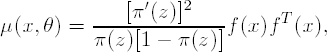
The quantal logistic model provides an example where the statement of the generalized equivalence theorem, (7.6) and (7.7), admits a more "numerically-friendly" presentation. For example, the information matrix for a single observation can be written as μ(x,θ) = g(x,θ)gT(x,θ), where

which, together with the matrix identity tr(AB) = tr(BA), leads to the following presentation of the sensitivity functions for the quantal model:
7.2.2. Example 1: A Two-Parameter Logistic Model
In this subsection we will take a closer look at the logistic model with two unknown parameters:
where θ1 and θ2 and the intercept and slope parameters, respectively.
It can be shown that D-optimal designs associated with the described model are two-point designs, with half the measurements at each dose, i.e., w1 = w2 = 0.5 (White, 1975). It is interesting to note that, when the dose range is sufficiently wide, D-optimal designs are uniquely defined in the z-space and the optimal design points correspond to certain response probabilities. Specifically, the optimal design points on the z scale are zopt = ∓1.543 and the corresponding response probabilities are given by
where π(z) = ez/(1 + ez). Thus, if x1* and x2* are the two optimal doses corresponding to a D-optimal design, then
It is also worth pointing out that, if xp is a dose level that causes a particular response in 100p of subjects, i.e., η(xp,θ) = p, the normalized variance of the MLE ![]() p in the two-parameter logistic model is a special case of the c-optimality criterion and can be written as
p in the two-parameter logistic model is a special case of the c-optimality criterion and can be written as
(Wu, 1988) with cp = f(xp)/θ2. For a discussion of c- and A-optimal designs for binary models, see Ford, Torsney and Wu (1992), Sitter and Wu (1993).
7.2.2.1. Illustration
Assume that the true values of the two parameters in the logistic model are θ1 = 1 and θ2 = 3. Assume also that the admissible dose range (design region) is given by χ = xmin, xmax with xmin = −1 and xmax = 1. First of all, note that
and therefore the D-optimal dose levels lie inside the design region. The optimal doses, (x1*,x2*), are found from
It is easy to verify that x1* = −0.848 and x2* = 0.181. The associated weights are w1 = w2 = 0.5.
7.2.2.2. Computation of the D-Optimal Design
This subsection introduces the %OptimalDesign1 macro that implements the optimal design algorithm in the univariate case (a single design variable x) and illustrates the process of computing a D-optimal design for the two-parameter logistic model described above. The advantage of using this simple model is that one can easily check individual elements of the resulting optimal design, including the information matrix, optimal doses and weights.
The %OptimalDesign1 macro supports two main components of the optimal design algorithm:
Calculation of the information matrix (%deriv and %infod macros).
Implementation of the forward and backward steps of the algorithm (%doptimal macro).
The first component (information matrix) in this list is model-specific whereas the second component (algorithm) does not depend on the chosen model. Note that the first component is the critical (and most computationally intensive) step in this macro.
Program 7.1 invokes the %OptimalDesign1 macro to compute a D-optimal design for the two-parameter logistic model. To save space, the complete SAS code is provided on the book's companion web site. This subsection focuses on the user-specified parameters that define the design problem and set up the optimal design algorithm.
The first four macro variables in Program 7.1 define the following design parameters:
POINTS is a vector of doses included in the initial design. In this case, the initial design contains four dose levels evenly spaced across the dose range χ = [−1,1].
WEIGHTS defines the weights of the four doses in the initial design (the doses are equally weighted).
GRID defines the grid points in the optimal design algorithm. The grid consists of 201 equally spaced points in the dose range. The DO function of the SAS/IML creates a list of equally spaced points. In this case, Do produces the following row vector, {−1, −0.99, −0.98,..., 0.98, 0.99,1}.
PARAMETER is a vector of model parameters. The true values of θ1 and θ2 are assumed to be 1 and 3, respectively.
The other five macro variables define the algorithm properties of the optimal design algorithm:
CONVC is the convergence criterion. It determines when the iterative procedure terminates.
MAXIMIT is the maximum number of iterations. A typical value of MAXIMIT is 200. A greater value is recommended when the final design is expected to contain a large number of points.
CONST1 and CONST2 are used in the calculation of weights in the optimal design algorithm (Section 7.1.5). By default, these constants are set to 1. The user can change these values to facilitate the convergence of the algorithm in models with a large number of parameters.
CMERGE is the merging constant in the optimal design algorithm that influences the process of merging design points. The default value of CMERGE is 3 and a larger value should be considered if the final design includes points with very small weights.
To calculate the information matrix μ(x,θ) and the sensitivity function ψ(x,ξ,θ), we needs to specify the g(x,θ) function introduced in Section 7.2.1. This function is defined in the %deriv macro. The MATRIX variable is the vector that contains the values of x, and the vector representing the g(x,θ) function is stored in the DERIVATIVE variable. In this case, the g(x,θ) function is given by
Example 7-1. D-optimal design for the two-parameter logistic model (Design parameters, algorithm parameters and g(x,θ) function)
* Design parameters;
%let points={−1 −0.333 0.333 1};
%let weights={0.25 0.25 0.25 0.25};
%let grid=do(−1,1,0.01);
%let parameter={1 3};
* Algorithm parameters;
%let convc=1e−7;
%let maximit=200;
%let const1=1;
%let const2=1;
%let cmerge=3;
* G function;
%macro deriv(matrix,derivative);
    nm=nrow(&matrix);
    one=j(nm,1,1);
    fm=one||&matrix;
    gc=exp(0.5*fm*t(parameter))/(1+exp(fm*t(parameter)));
    &derivative=gc#fm;
%mend deriv;
* Optimal design algorithm;
%OptimalDesign1; |
Example. Output from Program 7.1
Initial design

                                  Weight         X

                                   0.250    −1.000
                                   0.250    −0.333
                                   0.250     0.333
                                   0.250     1.000
Optimal design
Weight X
0.501 −0.850
0.499 0.180
Determinants of the variance-covariance matrices
INITIAL OPTIMAL
271.1 179.6
Variance-covariance matrix, initial design
COL1 COL2
11.0 9.2
9.2 32.4
Variance-covariance matrix, optimal design
COL1 COL2
9.8 8.7
8.7 26.0 |
The output produced by Program 7.1 includes the following data sets (Output 7.1):
INITIAL data set (design points and associated weights in the initial design).
OPTIMAL data set (design points and associated weights in the D-optimal design).
DDET data set (determinants of the variance-covariance matrix D(ξ,θ) for the initial and optimal designs).
DINITIAL data set (variance-covariance matrix D(ξ,θ) for the initial design).
DOPTIMAL data set (variance-covariance matrix D(ξ,θ) for the optimal design).
The program also creates two plots (Figure 7.3):
Plot of the initial and optimal designs.
Plot of the sensitivity functions associated with the initial and optimal designs.
Output 7.1 shows that the optimal doses are x1* = −0.85 and x2* = 0.18 with equal weights (see also the left panel in Figure 7.3). This example illustrates a well-known theoretical result that if a D-optimal design is supported at m points for a model with m unknown parameters, then the support points have equal weights, wi = 1/m, i = 1,...,m; see Fedorov (1972, Corollary to Theorem 2.3.1). It is easy to check that the optimal doses are very close to the doses we computed earlier from the equation zopt = ∓1.543.
We can also see from Output 7.1 that the determinant of the optimal variance-covariance matrix is 179.6 compared to the initial value of 271.1. There was also an improvement in the variance of the parameter estimates. The variance of ![]() 1 dropped from 11.0 to 9.8 and the variance of
1 dropped from 11.0 to 9.8 and the variance of ![]() 2 decreased from 32.4 to 26.0.
2 decreased from 32.4 to 26.0.
The right panel in Figure 7.3 shows that the equivalence theorem serves as an excellent diagnostic tool in optimization problems. The sensitivity function of the D-optimal design hits the reference line m = 2 at the optimal doses, i.e., at x = −0.85 and x = 0.18. For the D-criterion, the sensitivity function is identical to the normalized variance of prediction. Thus, since the sensitivity function of the initial design is greater than m = 2 at the left end of the dose range, we conclude that
Figure 7-3. Left panel: Initial (open circles) and optimal (closed circles) designs. Right panel: Sensitivity functions for the initial (dashed curve) and optimal (solid curve) designs.
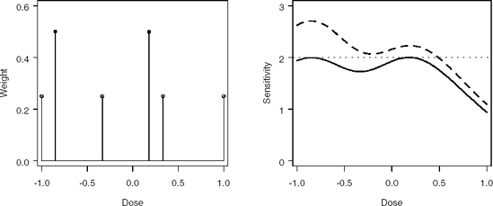
The initial design is not D-optimal.
More measurements should be placed at the left end of the design region in order to reduce the variance of prediction or, equivalently, push the sensitivity function down below the reference line defined by the equivalence theorem (m = 2).
7.2.3. Example 2: A Two-Parameter Logistic Model with a Narrow Dose Range
In Example 1, we considered the case when the admissible dose range was fairly wide, χ = [−1,1]. If the dose range is not sufficiently wide, at least one of the D-optimal points may coincide with the boundary and we will no longer be able to use the simple rule introduced earlier in this section (zopt = ∓1.543).
As an illustration, consider a narrower dose range, χ = [0,1]. To compute the D-optimal design for the two-parameter logistic model in this case, all we need to do is to modify the lower boundary of the dose range in Program 7.1. Program 7.2 derives the D-optimal design for the modified dose range (complete SAS code is given on the book's companion web site).
Example 7-2. D-optimal design for the two-parameter logistic model with a narrow dose range (Algorithm parameters and g(x,θ) function are identical to those defined in Program 7.1)
* Design parameters;
%let points={0 0.333 0.667 1};
%let weights={0.25 0.25 0.25 0.25};
%let grid=do(0,1,0.025);
%let parameter={1 3}; |
Example. Output 7.2
Initial design

                                  Weight         X

                                   0.250     0.000
                                   0.250     0.333
                                   0.250     0.667
                                   0.250     1.000

                                  Optimal design

                                  Weight         X

                                   0.500     0.000
0.500 0.725 |
Output 7.2 shows that the resulting D-optimal design is still a two-point design with equal weights w1 = w2 = 0.5; however, the optimal doses have changed. One dose is now located at the boundary of the region, x1* = 0, and the other dose has shifted to the right, x2* = 0.725 (see also Figure 7.4). As was pointed out in Section 7.1.5, optimal designs depend not only on the information matrix (which is identical to the information matrix in Example 1) but also on the dose range or, in general, design region.
Figure 7-4. Left panel: Initial (open circles) and optimal (closed circles) designs. Right panel: Sensitivity functions for the initial (dashed curve) and optimal (solid curve) designs.
