
2.3. Boosting
Several authors have written thorough summaries of the historical development of boosting (see, e.g., Friedman et al., 2000; Schapire, 2002) For completeness of this work, we provide a brief overview of boosting and include recent findings.
2.3.1. Evolution of boosting
The concept of boosting originated in the machine learning community where Kearns and Valiant (1989) explored weak learning algorithms (algorithms that can classify objects better than random) and strong learning algorithms (algorithms that can classify accurately). The question of the relationship between weak and strong learning algorithms was initially posed, and was addressed soon after by Schapire (1990). In his work, Schapire showed that if a concept was weakly learnable it was also strongly learnable and he formulated the first algorithm to "boost" a weak learner into a strong learner. Freund (1995) improved upon Schapire's initial algorithm by reducing its complexity and increasingits efficiency. However, both Schapire's algorithm and Freund's algorithms were difficult to implement in practice.
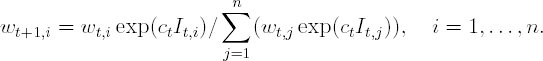
To overcome these practical implementation problems, Freund and Schapire (1996a) collaborated to produce the well-known and widely applied AdaBoost algorithm described below (the notation used in this algorithm is defined in Table 2.1).
Let w1,1 = ... =w1,n = 1/n.
For t = 1,2, ...,T do:
Fit ft using the weights, wt,1,...,wt,n, and compute the error, et.
Compute ct = ln((1 – et)/et).
Update the observation weights:
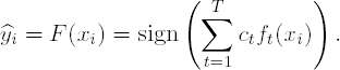
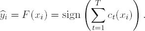
Output the final classifier:
| i | Observation number, i = 1,2, ...,n. |
| t | Stage number, t = 1,2, ...,T. |
| xi | A p-dimensional vector containing the quantitative variables of the ith observation. |
| yi | A scalar quantity representing the class membership of the ith observation, yi = −1 or 1. |
| ft | The weak classifier at the tth stage. |
| ft (xi) | The class estimate of the ith observation using the tth stage classifier |
| wt,i | The weight for the ith observation at the tth stage, Σi wt,i = 1. |
| It,i | Indicator function, I(ft (xi) ≠ yi). |
| et | The classification error at the tth stage, Σi wt,i It,i. |
| ct | The weight of ft. |
| sign(x) | = 1 if x ≥ 0 and = −1 otherwise. |
In short, AdaBoost generates a sequentially weighted additive agglomeration of weak classifiers. In each step of the sequence, AdaBoost attempts to find the best classifier according to the current distribution of observation weights. If an observation is incorrectly classified with the current distribution of weights, the observation receives more weight in the next sequence, while correctly classified observations receive less weight in the next iteration. In the final agglomeration, classifiers which are accurate predictors of the original data set receive more weight, whereas, weak classifiers that are poor predictors receive less weight. Thus, AdaBoost uses a sequence of simple weighted classifiers, each forced to learn a different aspect of the data, to generate a final, comprehensive classifier, which often classifies better than any individual classifier.
Friedman, Hastie and Tibshirani (2000) dissected the AdaBoost algorithm and revealed its statistical connections to loss functions, additive modeling, and logistic regression. Specifically, AdaBoost can be thought of as a forward stagewise additive model that seeks to minimize an exponential loss function:
- e−yF(x),
where F(x) denotes the boosted classifier (i.e., the classifier defined in Step 3 of the algorithm). Using this framework, Friedman, Hastie and Tibshirani (2000) generalized the AdaBoost algorithm to produce a real-valued prediction (Real AdaBoost) and corresponding numerically stable version (Gentle AdaBoost). In addition, they replaced the exponential loss function with a function more commonly used in the statistical field for binary data, the binomial log-likelihood loss function, and named this method LogitBoost. Table 2.2 provides a comparison of these methods.
2.3.1.1. Generalized Boosting Algorithm of Friedman, Hastie and Tibshirani (2000)
For t = 1,2, ...,T do:
Fit the model yiwork = f(xi using the weights, wt,i.
Compute ct(xi), a contribution of xi at stage t to the final classifier.
Update the weights, wt,i. Update yiwork (for LogitBoost only).
Output the final classifier:

|
2.3.2. Weak Learning Algorithms and Effectiveness of Boosting
As mentioned in the previous section, boosting can be applied to any classification method that classifies better than random. By far, the most popular and effective weaklearners are tree-based methods, also known as recursive partitioning. Several authors have provided explanations of why recursive partitioning can be boosted to produce effective classifiers (see, for example, Breiman, 1998). In short, boosting is effective for classifiers that are unstable (produce different models when given different training data from the same distribution), but when combined, get approximately the correct solution(i.e. have low bias). This breakdown is commonly known as the bias-variance trade-off (see, for example, Bauer and Kohavi, 1999). The importance of using an unstable classifiercan be easily seen by examining the AdaBoost algorithms further. Specifically, if a classifier misclassifies the same observations in consecutive iterations, then AdaBoost willbe prevented from finding additional structure in the data.
To explain further, let wt,i representthe weight of the ith observation at the tth stage of AdaBoost. Without loss of generality, suppose that the first m observations are misclassified and Σi=1n wt,i = 1. By the AdaBoost algorithm, the updated weights are

Next, suppose the first m observations are again misclassified in the (t+1)$st stage. Then,
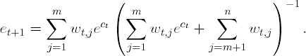
Notice that
Therefore, et+1 = 0.5 and ct+1 = 0. This implies that the weights for iteration t + 2 will be the same as the weights from iteration t + 1, and the algorithm will choose the same model. This fact will prevent the algorithm from learning any more about the relationship between the descriptor space and response classification. Hence, methods that are stable, such as linear discriminant analysis, k-nearest neighbors, and recursive partitions with many terminal nodes, will not be greatly improved by boosting. But, methods such as neural networks(Freund and Schapire, 1996b), Naive-Bayes (Bauer and Kohavi, 1999), and recursive partitions with few terminal nodes (also referred to as stumps) will be improved by boosting. For example, Optiz and Maclin (1999) compared boosting neural networks to boosting decision trees on twenty-three empirical data sets. For a majority of thedata sets, boosting neural networks or decision trees produced a more accurate classifier than any individual neural network or decision tree, respectively. However, Opitz and Maclin illustrated that the performance of boosting was data dependent; for several datasets a boosted neural network performed worse than an individual neural network. Additionally, Bauer and Kohavi (1999) illustrated that boosting a Naive-Bayes classifier improves classification, but can increase the variance of the prediction.
Because of the success of boosting with recursive partitioning with few terminal nodes, in the next section we will explore the implementation of boosting using stumps, arecursive partition with one split.
2.3.3. Implementation of Boosting in SAS
There are at least two ways to implement boosting in SAS. Conveniently, boosting can be directly implemented in SAS Enterprise Miner software. However, the use of SAS Enterprise Miner requires the purchase of this module. Boosting can also be implemented through more commonly and widely available SAS software such as Base SAS, SAS/STAT, and SAS/IML. This section will focus on the development of boosting code using widely available SAS modules. But, we begin this section by exploring a few details of boosting in SAS Enterprise Miner.
2.3.4. Implementation with SAS Enterprise Miner
In SAS Enterprise Miner, an ensemble classifier is quite easy to create, and can be generated with a minimum of four nodes (see Table 2.3). SAS documentation provides thorough step-by-step tutorial for creating various ensembles of classifiers in the Ensemble Node Help section; we refer you to this section for details on how to implement an ensemble model. Here, we highlight a few key facts about boosting in SAS Enterprise Miner.
| Node | Options |
|---|---|
| 1. Input Data Source | Select target (response) variable |
| 2. Group Processing | Mode = Weighted resampling for boosting |
| 3. Model | Select Tree model for a boosted recursive partition |
| 4. Ensemble | Ensemble node = Boosting |
To generate an ensemble model, the software requires the Input Data Source, Group Processing, Model, and Ensemble nodes. In the General Tab under Group Processing, one must select Weighted resampling for boosting and must specify the number of loops (iterations) to perform. Then, in the ensemble node, boosting must be chosen as the setting. It is important to note that SAS Enterprise Miner performs boosting by building trees on weighted resamples of the observations rather than buildings trees based on weighted observations. This typeof boosting is more commonly referred to as adaptive resampling and combining (ARCing) and was developed by Breiman (1998). In fact, the SAS Enterprise Miner implementation of boosting is only a slight modification of Breiman's Arc-x4 algorithm. While boosting andARCing have the same general flavor, Friedman, Hastie and Tibshirani (2000) indicate that boosting via weighted trees generally performs better than ARCing. Hence, a distinction should be made between the two methods.
Unfortunately, the constructs within SAS Enterprise Miner make it extremely difficult to implement boosting with weighted trees and any of the boosting algorithms from Table 2.2. Instead, we implement the generalized boosting algorithms directly through more commonly used SAS software.
2.3.5. Implementation of Boosting in Base SAS
For our implementation of boosting, we will use stumps—recursive partitions with one split—as the weak learner. We begin this section by focusing on the construction of code to find an optimal recursive partition in a set of data.
EXAMPLE: Recursive partitioning
Recursive partitioning seeks to find successive partitions of the descriptor spacethat separate the observations into regions (or nodes) of increasingly higher purity of the response. As an illustration, consider a data set that contains 100 four-dimensionalpoints,(x1,x2,y,w), where y is the class identifier and w is the weight. The data set is generated by Program 2.2. A plot of the generated data points is displayed in Figure 2.1.
Example 2-2. Simulated data in the recursive partitioning example
data example1;
    do i=1 to 100;
        x1 = 10*ranuni(1);
        x2 = 10*ranuni(2);
        if (x1<5 and x2<1.5) then y=0;
        if (x1<5 and x2>=1.5) then y=1;
        if (x1>=5 and x2<7.5) then y=0;
        if (x1<=5 and x2<=7.5) then y=1;
        w=1;
        output;
    end;
* Vertical axis;
axis1 minor=none label=(angle=90 "X2") order=(0 to 10 by 1) width=1;
* Horizontal axis;
axis2 minor=none label=("X1") order=(0 to 10 by 1) width=1;
symbol1 i=none value=circle color=black height=4;
symbol2 i=none value=dot color=black height=4;
proc gplot data=example1;
    plot x2*x1=y/vaxis=axis1 haxis=axis2 frame nolegend;
    run;
quit; |
Figure 2-1. Plot of the data in the recursive partitioning example

For this example, we desire to find a single partition of the data that creates two new regions of highest possible purity. Of course, the best partition is dependent on the measure of region impurity. An intuitive measure of impurity is misclassification error, but a more accepted impurity measure is the Gini Index. Let pj represent the proportion of observations of Class j in a node. For a two-class problem, the misclassification error of a node is defined as min(p1,p2), and the Gini Index is defined as 2p1p2. The total measure of impurity is a weighted sum of the impurity from each node, where each node is weighted by the proportion of observations in that node, relative to the total number of observations from its parent node.
For the EXAMPLE1 data set, a few possible partitions clearly stand out (see Figure 2.1):
- x1 = 5, x2 = 7.5 or x2 = 1.5.
Classification using these cut-points yields the results in Table 2.4. The corresponding measures of misclassification error and Gini Index can be found in Table 2.5.
| Class | x1 ≥ 5 | x1 < 5 | x2 < 7.5 | x2 ≥ 7.5 | x2 < 1.5 | x2 ≥ 1.5 |
|---|---|---|---|---|---|---|
| y = 0 | 40 | 11 | 51 | 0 | 14 | 37 |
| y = 1 | 7 | 42 | 32 | 17 | 0 | 49 |
| Partition | Misclassification error | Gini index |
|---|---|---|
| x1 ≥ 5 | min(7/47,40/47) = 0.15 | 2(7/47)(40/47) = 0.25 |
| x1 < 5 | min(11/53,42/53) = 0.21 | 2(11/53)(42/53) = 0.33 |
| Total | (0.47)(0.15) + (0.53)(0.21) = 0.18 | (0.47)(0.25) + (0.53)(0.33) = 0.29 |
| x2 ≥ 7.5 | min(32/83,51/83) = 0.39 | 2(32/83)(51/83) = 0.47 |
| x2 < 7.5 | min(0/17,17/17) = 0 | 2(0/17)(17/17) = 0 |
| Total | (0.83)(0.39) + (0.17)(0) = 0.32 | (0.83)(0.47) + (0.17)(0) = 0.39 |
| x2 ≥ 1.5 | min(37/86,49/86) = 0.43 | 2(37/86)(49/86) = 0.49 |
| x2 < 1.5 | min(0/14,14/14) = 0 | 2(0/14)(14/14) = 0 |
| Total | (0.14)(0) + (0.86)(0.43) = 0.37 | (0.14)(0) + (0.86)(0.49) = 0.42 |
Table 2.5 shows that the partition at x1 = 5 yields the minimum value for both total misclassification error (0.18) and the Gini index (0.29).
2.3.5.1. Unequally Weighted Observations
As defined above, misclassification error and Gini Index assume that each observation is equally weighted in determining the partition. These measures can also be computed for unequally weighted data. Define
Then for the two-class problem the misclassification error and Gini Index are min(p1*, p2*) and 2p1*p2*, respectively.
While three partitions for the EXAMPLE1 data set visually stand out in Figure 2.1, there are 198 possible partitions of this data. In general, the number of possible partitions for any data set is the number of dimensions multiplied by one fewer than the number of observations. And, to find the optimal partition one must search through all possible partitions. Using data steps and procedures, we can construct basic SAS code to exhaustively search for the best partition using the impurity measure of our choice, and allowing for unequally weighted data.
2.3.5.2. %Split Macro
The %Split macro searches for the optimal partition using the Gini index (the macro is given on the companion Web site). The input parameters for %Split are INPUTDS and P. The INPUTDS parameter references the data set for which the optimal split will be found, and this data set must have independent descriptors named X1, X2, ..., XP, a variable named W that provides each observation weight, and a response variable named Y that takes values 0 and 1 for each class. The user must also specify the P parameter, the number ofindependent descriptors. Upon calling %Split, it produces an output data set named OUTSPLIT that contains the name of the variable and split point that minimizes the Gini Index.
Program 2.3 calls the %Split macro to find the optimal binary split in the EXAMPLE1 data set using the Gini index.
Example 2-3. Optimal binary split in the recursive partitioning example
%split(inputds=example1,p=2);
proc print data=outsplit noobs label;
    format gini cutoff 6.3;
run; |
Example. Output from Program 2.3
Gini      Best       Best
                      index    variable    cutoff

0.293 x1 5.013 |
Output 2.3 output identifies x1 = 5.013 as the split that minimizes the Gini index. The Gini index associated with the optimalbinary split is 0.293.
While the %Split macro is effective for finding partitions of small data sets, itslooping scheme is inefficient. Instead of employing data steps and procedures to search for the optimal split, we have implemented a search module named IML_SPLIT that is basedon SAS/IML and that replaces the observation loop with a small series of efficient matrix operations.
2.3.5.3. AdaBoost Using the IML_SPLIT Module
The AdaBoost algorithm described in Section 2.3.1 is relatively easy to implement using the IML_SPLIT module as the weak learner (see the %AdaBoost macro on the book's companion Web site). Like the %Split macro, %AdaBoost has input parameters of INPUTDS and P, as well as ITER which specifies the number of boosting iterationsto perform. %AdaBoost creates a data set called BOOST that contains information about each boosting iteration. The output variables included in the BOOST data set are defined below.
ITER is the boosting iteration number.
GINI_VAR is the descriptor number at the current iteration that minimizes the Gini index.
GINI_CUT is the cut-point that minimizes the Gini Index.
P0_LH is the probability of class 0 for observations less than GINI_CUT.
P1_LH is the probability of class 1 for observations less than GINI_CUT.
C_L is the class label for observations less than GINI_CUT.
P0_RH is the probability of class 0 for observations greater than GINI_CUT.
P1_RH is the probability of class 1 for observations greater than GINI_CUT.
C_R is the class label for observations greater than GINI_CUT.
ALPHA is the weight of the cut-point rule at the current boosting iteration.
ERROR is the misclassification error of the cumulative boosting model atthe current iteration.
KAPPA is the kappa statistic of the cumulative boosting model at the current iteration.
To illustrate the %AdaBoost macro, again consider the EXAMPLE1 data set. Program 2.4 calls %AdaBoost to classify this data set using ten iterations. The program also produces plots of the misclassification error and kappa statistics for each iteration.
Example 2-4. AdaBoost algorithm in the recursive partitioning example
%AdaBoost(inputds=example1,p=2,iter=10);
proc print data=boost noobs label;
    format gini_cut p0_lh p1_lh p0_rh p1_rh c_r alpha error kappa 6.3;
    run;
* Misclassification error;
* Vertical axis;
axis1 minor=none label=(angle=90 "Error") order=(0 to 0.3 by 0.1) width=1;
* Horizontal axis;
axis2 minor=none label=("Iteration") order=(1 to 10 by 1) width=1;
symbol1 i=join value=none color=black width=5;
proc gplot data=boost;
    plot error*iter/vaxis=axis1 haxis=axis2 frame;
    run;
    quit;
* Kappa statistic;
* Vertical axis;
axis1 minor=none label=(angle=90 "Kappa") order=(0.5 to 1 by 0.1) width=1;
* Horizontal axis;
axis2 minor=none label=("Iteration") order=(1 to 10 by 1) width=1;
symbol1 i=join value=none color=black width=5;
proc gplot data=boost;
    plot kappa*iter/vaxis=axis1 haxis=axis2 frame;
    run;
quit; |
Example. Output from Program 2.4
iter gini_var gini_cut  p0_LH  p1_LH c_L  p0_RH  p1_RH    c_R  alpha  error  kappa

      1      1      5.013   0.208  0.792  1   0.851  0.149  0.000  1.516  0.180  0.640
      2      2      6.137   0.825  0.175  0   0.082  0.918  1.000  1.813  0.230  0.537
      3      2      1.749   1.000  0.000  0   0.267  0.733  1.000  1.295  0.050  0.900
      4      1      5.013   0.272  0.728  1   0.877  0.123  0.000  1.481  0.050  0.900
      5      2      7.395   0.784  0.216  0   0.000  1.000  1.000  1.579  0.000  1.000
      6      2      1.749   1.000  0.000  0   0.228  0.772  1.000  1.482  0.050  0.900
      7      1      5.013   0.266  0.734  1   0.875  0.125  0.000  1.483  0.000  1.000
      8      2      7.395   0.765  0.235  0   0.000  1.000  1.000  1.462  0.000  1.000
      9      2      1.749   1.000  0.000  0   0.233  0.767  1.000  1.457  0.000  1.000
10 1 5.013 0.273 0.727 1 0.871 0.129 0.000 1.451 0.000 1.000 |
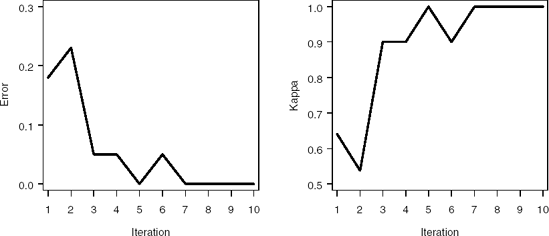
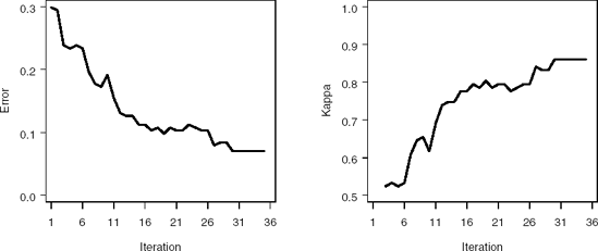
Output 2.4 lists the BOOST data set generated by the %AdaBoost macro. For the first iteration, x1 minimizes the Gini index at 5.013. For observations with x1 < 5.013, the probability of observing an observation in Class 0 is 0.208, while the probability of observing an observation in Class 1 is 0.792. Hence the class label for observations taking values of x1 < 5.013 is 1. Similarly, for observations with x1 > 5.013, the probability of observing an observation in the Class 0 and 1 are 0.851 and 0.149, respctively. Therefore, the class label for observations taking values of x1 > 5.013 is 0. The stage weight for the first boosting iteration is represented by ALPHA = 1.516, while the observed classification error and kappastatistics are 0.18 and 0.64, respectively. Notice that the AdaBoost algorithm learns the structure of the relationship between the descriptor space and classification vector in saven iterations (the misclassification error and kappa statistic displayed in Figure 2.2 reach a plateau by the seventh iteration), and in these iterations the algorithm quickly identifies cut-points near the constructed splits of x1 = 5, x2 = 7.5 and x2 = 1.5.
Figure 2-2. Misclassification error (left panel) and kappa statistic (right panel) plots for the EXAMPLE1 data set using the %AdaBoost macro
Program 2.5 models the permeability data of Section 2.2 with AdaBoost and plots the misclassification error and kappa statistics at each iteration.
Example 2-5. AdaBoost algorithm in the permeability data example
%AdaBoost(inputds=permy,p=71,iter=50);
proc print data=boost noobs label;
    format gini_cut p0_lh p1_lh p0_rh p1_rh c_r alpha error kappa 6.3;
    run;
* Misclassification error;
* Vertical axis;
axis1 minor=none label=(angle=90 "Error") order=(0 to 0.3 by 0.1) width=1;
* Horizontal axis;
axis2 minor=none label=("Iteration") order=(1 to 51 by 10) width=1;
symbol1 i=join value=none color=black width=5;
proc gplot data=boost;
    plot error*iter/vaxis=axis1 haxis=axis2 frame;
    run;
    quit;
* Kappa statistic;
* Vertical axis;
axis1 minor=none label=(angle=90 "Kappa") order=(0.5 to 1 by 0.1) width=1;
* Horizontal axis;
axis2 minor=none label=("Iteration") order=(1 to 51 by 10) width=1;
symbol1 i=join value=none color=black width=5;
proc gplot data=boost;
    plot kappa*iter/vaxis=axis1 haxis=axis2 frame;
    run;
quit; |
Example. Output from Program 2.5
iter gini_var gini_cut  p0_LH  p1_LH c_L  p0_RH  p1_RH    c_R  alpha  error  kappa

      1      6     1029.7   0.294  0.706  1   0.706  0.294  0.000  0.877  0.294  0.412
      2     68     82.813   0.436  0.564  1   0.805  0.195  0.000  0.431  0.294  0.412
      3     33      0.992   0.129  0.871  1   0.603  0.397  0.000  0.493  0.268  0.463
      4     69     45.125   0.437  0.563  1   0.940  0.060  0.000  0.335  0.274  0.452
      5     37     63.938   0.356  0.644  1   0.603  0.397  0.000  0.462  0.271  0.458
      6     24      0.493   0.419  0.581  1   0.704  0.296  0.000  0.443  0.249  0.503
      7     43     22.930   0.448  0.552  1   0.654  0.346  0.000  0.407  0.254  0.492
      8     28      0.012   0.639  0.361  0   0.403  0.597  1.000  0.392  0.246  0.508
      9     23      1.369   0.496  0.504  1   0.961  0.039  0.000  0.111  0.246  0.508
     10     20      1.641   0.565  0.435  0   0.000  1.000  1.000  0.320  0.249  0.503
     11     23      1.369   0.449  0.551  1   0.957  0.043  0.000  0.276  0.240  0.520
     12      3      1.429   0.263  0.737  1   0.569  0.431  0.000  0.320  0.251  0.497
     13     69     45.125   0.452  0.548  1   0.924  0.076  0.000  0.252  0.240  0.520
     14     34      5.454   0.469  0.531  1   0.672  0.328  0.000  0.297  0.226  0.548
     15     31      7.552   0.529  0.471  0   0.842  0.158  0.000  0.246  0.226  0.548
     16     31      7.552   0.468  0.532  1   0.806  0.194  0.000  0.234  0.220  0.559
     17     32      8.937   0.572  0.428  0   0.228  0.772  1.000  0.348  0.215  0.571
     18     23      1.369   0.455  0.545  1   0.966  0.034  0.000  0.244  0.206  0.588
     19     20      0.836   0.615  0.385  0   0.442  0.558  1.000  0.352  0.223  0.554
     20     63     321.50   0.633  0.367  0   0.447  0.553  1.000  0.357  0.189  0.621
     21     68     77.250   0.488  0.512  1   0.727  0.273  0.000  0.212  0.203  0.593
     22     59     46.250   0.589  0.411  0   0.159  0.841  1.000  0.400  0.201  0.599
     23     23      1.369   0.463  0.537  1   0.954  0.046  0.000  0.209  0.189  0.621
     24      7     736.00   0.499  0.501  1   0.768  0.232  0.000  0.126  0.192  0.616
     25     42      8.750   0.363  0.637  1   0.591  0.409  0.000  0.362  0.189  0.621
     26     52      1.872   0.447  0.553  1   0.654  0.346  0.000  0.309  0.192  0.616
27 61 −1.348 0.300 0.700 1 0.564 0.436 0.000 0.317 0.189 0.621
28 57 278.81 0.450 0.550 1 0.747 0.253 0.000 0.266 0.178 0.644
29 59 46.250 0.547 0.453 0 0.107 0.893 1.000 0.243 0.172 0.655
30 25 0.092 0.868 0.132 0 0.457 0.543 1.000 0.223 0.167 0.667
31 36 206.13 0.545 0.455 0 0.184 0.816 1.000 0.242 0.164 0.672
32 47 23.103 0.696 0.304 0 0.443 0.557 1.000 0.290 0.172 0.655
33 4 1.704 0.501 0.499 0 0.766 0.234 0.000 0.112 0.167 0.667
34 4 1.704 0.474 0.526 1 0.745 0.255 0.000 0.186 0.175 0.650
35 20 1.641 0.549 0.451 0 0.000 1.000 1.000 0.236 0.158 0.684
36 23 1.369 0.466 0.534 1 0.946 0.054 0.000 0.186 0.169 0.661
37 62 −0.869 0.262 0.738 1 0.548 0.452 0.000 0.254 0.150 0.701
38 6 1279.9 0.455 0.545 1 0.812 0.188 0.000 0.233 0.164 0.672
39 32 6.819 0.559 0.441 0 0.355 0.645 1.000 0.267 0.158 0.684
40 32 0.707 0.305 0.695 1 0.520 0.480 0.000 0.094 0.164 0.672
41 29 7.124 0.568 0.432 0 0.403 0.597 1.000 0.347 0.138 0.723
42 12 2.000 0.218 0.782 1 0.521 0.479 0.000 0.194 0.138 0.723
43 31 7.552 0.420 0.580 1 0.737 0.263 0.000 0.381 0.150 0.701
44 33 0.992 0.183 0.817 1 0.546 0.454 0.000 0.245 0.133 0.734
45 23 1.369 0.459 0.541 1 0.932 0.068 0.000 0.208 0.141 0.718
46 55 975.56 0.236 0.764 1 0.541 0.459 0.000 0.227 0.136 0.729
47 53 18.687 0.564 0.436 0 0.411 0.589 1.000 0.320 0.127 0.746
48 35 249.00 0.371 0.629 1 0.573 0.427 0.000 0.391 0.130 0.740
49 7 736.00 0.442 0.558 1 0.730 0.270 0.000 0.304 0.124 0.751
50 48 60.067 0.451 0.549 1 0.606 0.394 0.000 0.319 0.138 0.723 |
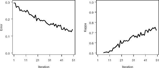
Output 2.5 provides important information for the progress of the algorithm for each iteration. Is shows that in the first 50 iterations, variable X23 is selected six times, while X20, X31, and X32 are selected three times each; boosting is focusing on variables that are important for separating the data into classes. Also, a number of variables are not selected in any iteration.
Figure 2.3 displays the error and kappa functions. Notice that after approximately35 iterations, the error levels off at approximately 0.15. At this point, AdaBoost is learning the training data at a much slower rate.
Figure 2-3. Misclassification error (left panel) and kappa statistic (right panel)plots for the PERMY data set using the %AdaBoost macro
2.3.6. Implementation of Generalized Boosting Algorithms
In most model building applications, we need to evaluate the model's performance on an independent set of data. This process is referred to as validation or cross-validation. In this section we provide a more general macro, %Boost, that can be used to evaluate both training and testing data. This macro also implements the other generalized forms of boosting.
The generalized boosting algorithms described in Section 2.3.1 can be implemented using the same structure of the %AdaBoost macro by making several appropriate adjustments. To implement the Real AdaBoost algorithm, we must use predicted class probabilities in place of predicted classification, and alter the observation contributions and weights. Because the %Split macro generates predicted class probabilities, we can directly construct Real AdaBoost. However, both Gentle AdaBoost and LogitBoost require a method that predicts a continuous, real-valued response. This stipulation requires that we implementa different form of recursive partitioning. Instead of using partitioning based on a categorical response, we will implement partitioning based on a continuous response. In short, we seek to find the partition that minimizes the corrected sum-of-squares, rather than misclassification error or Gini Index, of the response across both new nodes. That is, we seek the variable, xj, and cut-point, c, that minimize
where r1j = {i: xj < c} and r2j = {i: xj ≥ c}.
Like partitioning based on a categorical response, partitioning based on a continuous response requires an exhaustive search to find the optimal cut-point. To find the variable and optimal cut-point, we have created a SAS/IML module, REGSPLIT_IML. This module is included in our comprehensive macro, %Boost, that implements the AdaBoost, Real AdaBoost, Gentle AdaBoost, and LogitBoost algorithms (the macro is provided on the book's companion Web site). The input variables for %Boost are the same as %AdaBoost. In addition, the user must specify the type of boosting to perform (TYPE=1 performs AdaBoost, TYPE=2 performs Real AdaBoost, TYPE=3 performs Gentle AdaBoost, and TYPE=4 performs LogitBoost). When AdaBoost or Real AdaBoost are requested, %Boost produces an output data set with the same output variables as the AdaBoost macro. However, if Gentle AdaBoost or LogitBoost are specified, then a different output data set is created. The variables incuded in this data set are listed below.
ITER is the boosting iteration number.
REG_VAR is the variable number that minimizes the corrected sum-of-squares.
MIN_CSS is the minimum corrected sum-of-squares.
CUT_VAL is the optimal cut-point.
YPRED_L is the predicted value for observations less than CUT_VAL.
YPRED_R is the predicted value for observations greater than CUT_VAL.
ERROR is the misclassification error of the cumulative boosting model at the current iteration.
KAPPA is the kappa statistic of the cumulative boosting model at the current iteration.
As a diagnostic tool, the %Boost macro also creates an output data set named OUTWTS that contains observation weights at the final boosting iteration. These can be used to identify observations that are difficult to classify.
To illustrate the %Boost macro, Program 2.6 analyzes the EXAMPLE1 data set using the Gentle AdaBoost algorithm with 10 iterations.
Example 2-6. Gentle AdaBoost algorithm in the recursive partitioning example
%boost(inputds=example1,p=2,outputds=out_ex1,outwts=out_wt1,iter=10,type=3);
proc print data=out_ex1 noobs label;
    format min_css cut_val ypred_l ypred_r error kappa 6.3;
proc print data=out_wt1;
    format weight 7.5;
run; |
Example. Output from Program 2.6
OUT_EX1 data set

  iter  reg_var  min_css  cut_val  ypred_L  ypred_R   error   kappa

    1      1      0.587    5.013    0.585   −0.702    0.180   0.640
    2      2      0.528    6.137   −0.574    0.835    0.160   0.682
    3      2      0.679    1.749   −1.000    0.357    0.050   0.900
    4      1      0.600    5.013    0.603   −0.656    0.070   0.860
    5      2      0.627    7.395   −0.388    1.000    0.000   1.000
    6      2      0.702    1.749   −1.000    0.365    0.000   1.000
    7      1      0.577    5.013    0.639   −0.659    0.000   1.000
    8      2      0.669    7.395   −0.343    1.000    0.000   1.000
    9      2      0.722    1.749   −1.000    0.343    0.000   1.000
   10      1      0.566    5.013    0.651   −0.665    0.000   1.000

                            OUT_WT1 data set

                            Obs     weight

                              1    0.00019
                              2    0.01207
                              3    0.03347
                              4    0.00609
                              5    0.01820
                              6    0.00609
                              7    0.00010
                              8    0.00609
                              9    0.00295
10 0.00609 |
Output 2.6 provides a listing of the data set produced by the %Boost macro (OUT_EX1 data set). For the first iteration, X1 minimizes the corrected sum-of-squares (0.587) at the cut-point of 5.013. Observations that are less than this value have a predicted value of 0.585, whereas observations greater than this value have a predicted value of −0.702. For Gentle AdaBoost, the error at the first iteration is 0.18, while the kappa value is 0.64.
In addition, Output 2.6 lists the first ten observations in the OUT_WT1 data set which includes the final weights for each observation after ten iterations. These weightsare constrained to sum to one; therefore, relatively high weights represent observationsthat are difficult to classify, and observations with low weights are relatively easy toclassify.
One can also model the permeability data using Gentle AdaBoost. But, first, we should split the data into training and testing sets in order to evaluate each model's performance on an independent set of data. For this chapter, the permeability data set has already been separated into training and testing sets through the SET variable. Program 2.7 creates the training and testing sets and invokes the %Boost macro to perform Gentle AdaBoost on the training data with 35 iterations.
Example 2-7. Gentle AdaBoost algorithm in the permeability data example
data train;
    set permy(where=(set="TRAIN"));
data test;
    set permy(where=(set="TEST"));
    run;
%boost(inputds=train,p=71,outputds=genout1,outwts=genwt1,iter=35,type=3);
proc print data=genout1 noobs label;
    format min_css ypred_l ypred_r error kappa 6.3;
    run;
* Misclassification error;
* Vertical axis;
axis1 minor=none label=(angle=90 "Error") order=(0 to 0.3 by 0.1) width=1;
* Horizontal axis;
axis2 minor=none label=("Iteration") order=(1 to 36 by 5) width=1;
symbol1 i=join value=none color=black width=5;
proc gplot data=genout1;
    plot error*iter/vaxis=axis1 haxis=axis2 frame;
    run;
    quit;
* Kappa statistic;
* Vertical axis;
axis1 minor=none label=(angle=90 "Kappa") order=(0.5 to 1 by 0.1) width=1;
* Horizontal axis;
axis2 minor=none label=("Iteration") order=(1 to 36 by 5) width=1;
symbol1 i=join value=none color=black width=5;
proc gplot data=genout1;
    plot kappa*iter/vaxis=axis1 haxis=axis2 frame;
    run;
quit; |
Example. Output from Program 2.7
iter  reg_var  min_css  cut_val  ypred_L  ypred_R   error   kappa

    1       6     0.838   1047.69   0.374   −0.434    0.299   0.402
    2      42     0.910      8.75   0.649   −0.142    0.294   0.411
    3      70     0.878     13.81   0.181   −0.734    0.238   0.523
    4      33     0.933      1.17   0.706   −0.116    0.234   0.533
    5      37     0.928     75.56   0.348   −0.201    0.238   0.523
    6       7     0.922    745.06   0.101   −0.803    0.234   0.533
    7      63     0.920    318.81  −0.325    0.241    0.196   0.607
    8      43     0.943     16.74   0.333   −0.172    0.178   0.645
    9      45     0.938     23.72  −0.464    0.136    0.173   0.654
   10      56     0.939    452.44   0.337   −0.186    0.192   0.617
   11      19     0.946      0.50  −0.349    0.157    0.154   0.692
   12      71     0.944    549.46  −0.078    0.751    0.131   0.738
   13      15     0.936      0.10   0.485   −0.122    0.126   0.748
   14      32     0.953      8.85  −0.057    0.716    0.126   0.748
   15      23     0.949      1.38   0.066   −0.924    0.112   0.776
   16       1     0.950    624.00   1.000   −0.065    0.112   0.776
   17      59     0.955     46.25  −0.037    0.849    0.103   0.794
   18      57     0.941    278.81   0.091   −0.738    0.107   0.785
   19      60     0.944      8.75  −0.142    0.424    0.098   0.804
   20      68     0.951     84.94   0.073   −0.704    0.107   0.785
   21      34     0.955      0.71  −0.539    0.074    0.103   0.794
22 41 0.950 9.88 0.747 −0.137 0.103 0.794 23 34 0.956 0.71 −0.518 0.095 0.112 0.776 24 33 0.949 0.99 0.724 −0.137 0.107 0.785 25 13 0.957 0.02 1.000 −0.036 0.103 0.794 26 57 0.959 274.63 0.085 −0.573 0.103 0.794 27 32 0.957 1.58 0.191 −0.224 0.079 0.841 28 34 0.947 0.71 −0.584 0.093 0.084 0.832 29 32 0.938 8.85 −0.148 0.856 0.084 0.832 30 34 0.951 0.71 −0.546 0.099 0.070 0.860 31 34 0.947 0.71 −0.612 0.000 0.070 0.860 32 34 0.947 0.71 −0.612 0.000 0.070 0.860 33 34 0.947 0.71 −0.612 −0.000 0.070 0.860 34 34 0.947 0.71 −0.612 −0.000 0.070 0.860 35 34 0.947 0.71 −0.612 −0.000 0.070 0.860 |
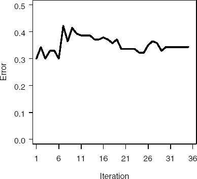
Output 2.7 lists the GENOUT1 data set created by the %Boost macro. Figure 2.4 illustrates the performance of the Gentle AdaBoost algorithm on the training data set. Notice that the training error decreases from 0.3 to around 0.1 after approximately 25 iterations.
Figure 2-4. Misclassification error (left panel) and kappa statistic (right panel) plots for the training subset of the PERMY data set using the %Boost macro (Gentle AdaBoost algorithm)
2.3.6.1. %Predict Macro
To complement the %Boost macro, we have also developed a macro, %Predict, to predict new observations using the model information generated by %Boost. This macro can be used to evaluate the performance of a model on an independent testing or validation data set. The input variables to %Predict are:
PRED_DS is the name of the data set to be predicted. This data set must have descriptors named X1, X2, ..., XP. The response must be named Y and must assume values of 0 or 1.
P is the number of descriptors in the input data set.
BOOST_DS is the name of the data set with boost model information (the OUTPUTDS from the %Boost macro).
TYPE is the type of boosting for prediction.
ITER is the number of boosting iterations desired.
Program 2.8 calls the %Predict macro to examine the predictive properties of the classification model in the permeability data example. The program analyzes the TEST data set created in Program 2.7.
Example 2-8. Prediction in the permeability data example
%predict(pred_ds=test,p=71,boost_ds=genout1,outputds=gentst1,out_pred=genpred1,
    type=3,iter=35);
* Misclassification error;
* Vertical axis;
axis1 minor=none label=(angle=90 "Error") order=(0 to 0.5 by 0.1) width=1;
* Horizontal axis;
axis2 minor=none label=("Iteration") order=(1 to 36 by 5) width=1;
symbol1 i=join value=none color=black width=5;
proc gplot data=gentst1;
    plot error*iter/vaxis=axis1 haxis=axis2 frame;
    run;
quit; |
Figure 2.5 depicts changes in the model error across iterations. Although we saw adecrease in the misclassification error for the training set across iterations (Figure 2.4), the same is not true for the test set. Instead, the misclassification error goes upslightly across iterations. For drug discovery data, this phenomenon is not surprising—often the response in many data sets is noisy (a number of samples have been misclassified). These misclassified samples hamper the learning ability of many models, preventing them from learning the correct structure between the descriptors and the classification variable. In Section 2.4, we further explain how to use boosting to identify noisy or mislabeled observations. Removing these observations often produces a better overall predictive model.
Figure 2-5. Misclassification rates in the testing subset of the PERMY data set using the %Predict macro (Gentle AdaBoost algorithm)
2.3.7. Properties of boosting
Many authors have shown that boosting is generally robust to overfitting; that is, as the complexity of the boosting model increases for the training set (i.e. the number of iterations increases), the test set error does not increase (Schapire, Freund, Bartlett and Lee, 1998; Friedman, Hastie, and Tibshirani, 2000; Freund, Mansour and Schapire, 2001). However, boosting, by its inherent construction, is vulnerable to certain types of data problems, which can make it difficult for boosting to find a model that can be generalized.
The primary known problem for boosting is noise in the response (Kriegar, Long andWyner, 2002; Schapire, 2002; Optiz and Maclin, 1999), which can occur when observationsare mislabeled or classes overlap in descriptor space. Under either of these circumstances, boosting will place increasing higher weights on those observations that are inconsistent with the majority of the data. As a check-valve, the performance of the model at each stage is evaluated against the original training set. Models that poorly classify receive less weight, while models that accurately classify receive more weight. But, the final agglomerative model has attempted to fit the noise in the response. Hence, the finalmodel will use these rules to predict new observations, thus increasing prediction error.
For similar reasons, boosting will be negatively affected by observations that areoutliers in the descriptor space. In fact, because of this problem, Freund and Schapire (2001) recommend removing known outliers before performing boosting.
Although noise can be an Achilles heal to boosting, its internal correction methods can help us identify potentially mislabeled or outlying observations. Specifically, asthe algorithm iterates, boosting will place increasing larger weights on observations that are difficult to classify. Hence, tracking observation weights can be used as a diagnostic tool for identifying these problematic observations. In the following section, we will illustrate the importance of examining observations weights.