6.4. Power Determination in a Purely Nonparametric Sense

The title of this section must seem a bit of an enigma. What does the expression "in a purely nonparametric sense" really mean? Let's begin by reviewing some basic concepts in experimental design and power in the familiar parametric sense. We will then demonstrate a nonparametric approach to the same setting. Lastly, we will compare and contrast the two approaches to highlight important features.

Consider the design of a simple two-group experiment. Subjects or samples are randomized to one of two groups and receive a treatment. After treatment, a measurement is collected and the investigators wish to see if evidence exists to declare the responses of the two groups to be "different".

What does it mean for two treatments to be different? Typically, the investigators are interested in finding a statistically significant effect at some level (say, 0.05) with some reasonable degree of certainty (say, at least 80% of the time). Using some common symbolism from mathematical statistics, the latter expression may be written as:

Test H₀ : μ₁ − μ₂ = 0 vesus H_A : μ₁ − μ₂ = δ at some level α,

where:

• α = P(Conclude μ₁ − μ₂ > 0 |(μ₁ − μ₂) = 0),

• 1 − β = P(Conclude μ₁ − μ₂ > 0|(μ₁ − μ₂) = δ).

In other words, we are interested in finding a statistically significant difference at an α level with 1 − β power when the true difference is δ. If we make the standard assumptions of two independent and identically distributed Gaussian samples (N(μ₁,σ²) and N(μ₂,σ²), respectively), we can perform such a comparison via a two-sample Student's t-test, i.e., reject H₀ in favor of H_A if

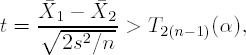
where ₁ and ₂ correspond to the sample means of Treatment Groups 1 and 2, respectively, s² is the pooled variance estimator, and T_2(n−1)(α) is a quantile from a standard Student's t-distribution with 2(n − 1) degrees of freedom.

Naturally, the investigators are interested in the total number of experimental units or subjects, 2n, required to conduct the experiment. The sample size per group, n, may be determined iteratively, using a standard inequality:

where T_2(n−1)(α) and T_2(n−1)(β) are quantiles from a standard Student's t-distribution with 2(n − 1) degrees of freedom.

Note the key features of this method of sample size determination are

• The person using this method needs to feel fairly confident that his or her measure comes from a distribution that is Gaussian (normal).

• He or she must have a reasonable idea of what the treatment effect should be.

• He or she must also have a reasonable estimate of the spread or dispersion of the desired effect (s²).

It is generally difficult for scientific investigators (based on the author's personal experience in statistical consulting) to provide information about a measurement's distribution. In fact, it is sometimes very difficult in some scientific disciplines (e.g., toxicology) for investigators to predict the size of effect that will be elicited by a treatment a priori.

One possible way to solve this problem is to conduct a small pilot study to get some initial intuition about a measurement's properties. Such a study will provide investigators with insight into the size of treatment effect that is achievable, as well as some preliminary ideas about the measurement's properties, such as its pattern of dispersion. However, will such a study address the fundamental question of distribution (e.g., Gaussian distribution) when the sample size is small?

A distribution-free, or nonparametric, approach to sample size estimation frees scientists from guessing about the distribution of measurement or treatment effect. One common way to estimate a sample size in a study with two independent groups, suggested by Collings and Hamilton (1988), requires that investigators perform a small pilot study. Investigators then use the pilot study's results to refine their estimates of achievable treatment effect. The scientists must also provide an estimate of their desired statistical significance level; however, they do not have to have any estimate of the dispersion or variation of the measurement at the time of the sample size determination. This information can be indirectly gleaned from the pilot study. For a given pair of sample sizes, say, n₁ and n₂, scientists determine the level of power associated with the comparison.

6.4.1. Power Calculations in a Two-Sample Case

How does the Collings-Hamilton technique work? Suppose the pilot study consists of data from two groups, say, X₁,..., X_n1 and Y₁,..., Y_n2. For the moment, let's assume that n₁ = n₂ = n and thus the total pilot sample size is 2n observations. Suppose we are interested in determining the power of a comparison of two treatment groups' location parameters, one shifted by an amount δ from the other, at the α-level of statistical significance, with a total sample size of 2m (m samples per treatment group). We begin by making a random selection (with replacement) of size 2m from the pilot study data, i.e., X₁,..., X_n1, Y₁,..., Y_n2. Denote the first m randomly sampled observations by R₁,..., R_m. For the second set of randomly selected observations (denoted by R_m+1,..., R_2m), add the change in location, δ, to each of the m values. Denote the resulting values R_m+1 + δ,..., R_2m + δ by S₁,..., S_m. Now compare R₁,..., R_m with S₁,..., S_m via a form of two-sample location comparison test, with a statistic, say, W, at level α. Create an indicator variable, I, and let I = 1 if W ≥ c_α (c_α represents the α-level cutoff of the test) and 0 otherwise.

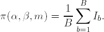
We can repeat the process B times (for some large value of B, i.e., B > 1000), recording the value of the indicator variable I as I_b for the bth repetition of the process (b = 1,..., B). An estimate of the power, π(α,β,m), of the test conducted at the α-level of significance, for shift of size and sample size m per group is

Collings and Hamilton went on to show in their paper that the described procedure can be improved in the following way. Consider X₁,..., X_n and randomly sample from the group 2_m times. For the second half of the 2m terms, add the shift value δ to each term: X_m+1 + δ,..., X_2m + δ. Perform the pair-wise comparison at level α between X₁,..., X_m and X_m+1 + δ,..., X_2m + δ, record the result via an indicator variable, and repeat the procedure B times, as described previously. The same procedure is carried out for Y₁,..., Y_n. Let π_X(α,β,m) be the power calculated for the X_i's and π_Y(α,β,m) be the power calculated for the Y_i's. The power for the comparison of X₁,..., X_n and Y₁,..., Y_n with respect to a shift δ, at level α, for total sample size 2m is:

Earlier in our discussion we assumed n₁ = n₂ = n. This condition is not necessary. If n₁ ≠ n₂, this approach can be modified by using a weighted mean of the two power values; see Collings and Hamilton (1988) for details.

6.4.2. Power Calculations in a k-Sample Case

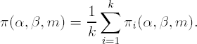
Mahoney and Magel (1996) extended the results of Collings and Hamilton to cover the case of k independent samples and their comparison by the Kruskal-Wallis test. The procedure is similar in spirit to that described previously. Consider the testing problem defined in Section 6.3, i.e., consider a study with k treatment groups and n_i units/subjects in the ith group. In the two-sample case, we talk about a single shift in location, δ. For a k-sample one-way layout, we have to talk about a k-dimensional vector, = (δ₁,..., δ_k), where δ_i is the shift-change in location of the ith group. Without loss of generality, we assume that the first delta component is zero, i.e., δ₁ = 0. As was the case in the two-sample setting, we again need to randomly sample (with replacement) from each of the groups. For the ith group, we sample km observations. We then apply the k location shifts to each of the km observations as follows. The first m observations are unshifted because δ₁ = 0. The second set of m observations are then shifted by δ₂, the third set by δ₃, etc. Mahoney and Magel point out that, essentially, we now have k random samples of size m, only differing by a shift in location and thus we can perform a Kruskal-Wallis test at level α. If the test is statistically significant, we let I₁ = 1, otherwise I₁ = 0. We repeat the process B times, for a large value of B, recording the value of I_b for the bth repetition of the process. The power for the ith group is calculated as before, i.e., π_i(α,β,m) = B⁻¹ Σ_b=1^B I_b. The outlined procedure is repeated for the remaining k − 1 groups and the power for the Kruskal-Wallis test is then simply the average power determined k times:

6.4.3. Comparison of Parametric and Nonparametric Approaches

Now is probably a good time to compare and contrast the parametric approach to sample size determination in a two-sample setting with the nonparametric approach. Notice we require some similar pieces of information in both approaches: we require knowledge about the level of the test, α, the desired effect, δ, and the number of observations per group, say, m. For the parametric comparison, we assume a common form of distribution for both groups, with an assumed known and identical scale parameter σ, and known location parameters (means) μ₁ and μ₂, respectively. The nonparametric approach requires a small pilot data set consisting of two groups without any assumptions about the common distributional form. For pharmaceutical researchers, the nonparametric approach may require more work because it requires data before the power may be calculated. However, the benefits of the procedure may greatly outweigh the expenditure of resources for the pilot.

First, investigators get to see the distribution of real data, as opposed to imagining what it would look like, conditional on a value of location and scale and assuming some pre-specified mathematically convenient form. Often investigators will use the summary statistics from a previously published manuscript to determine the power in the parametric approach for their investigation. Were the originally published data distributed normally? Were they symmetrically distributed, for that matter? We really do not know by looking at the summary statistics alone in the manuscript, nor can we learn much more if the authors made a poor choice of data visualization to summarize the paper's findings. We only know for certain about the raw data's features if we can see all of the data used in the original manuscript. It has been the author's experience that such data is difficult to get, as scientific writers change institutional affiliations and are subsequently difficult to locate years after they publish their research. Moreover, some are unwilling to share raw data, or unable to share it because of the proprietary nature of their research or because the data are stored in an inconvenient form (e.g., in several spreadsheets or laboratory notebooks).

Second, the nonparametric approach is intuitive, given that a scientist understands how the nonparametric test works. Power corresponds to the probability of, in some sense, finding a true and context meaningful difference, δ, at the α-level of significance for a given sample size. By employing the calculations described above, scientists can see where the value of power comes from without having to understand the mathematical statistical properties of the Gaussian (normal) distribution.

6.4.3.1. %KWSS Macro

How do we perform a nonparametric power analysis in SAS? The Mahoney-Magel generalization of the Collings-Hamilton approach to power determination in the k-sample setting may be accomplished with a SAS macro called %KWSS provided on the book's companion Web site. The %KWSS macro consists of a body of code containing one embedded macro (%BOOTSTRAP). The macro requires seven input parameters:

• IDSN is the name of an input SAS data set.

• GROUP is the grouping or classification variable.

• VAR is the response measurement variable.

• SHIFTLIST is the shift vector, = (δ₁,..., δ_k), for the test.

• SAMPLE_SIZE is the sample size for power determination.

• ITERATION_NO is the number of re-sampled data sets.

• ALPHA is the desired level of statistical significance.

The macro first removes any observations that contain a missing response. It then determines the number of groups in the input data set IDSN and creates a list of these groups with the macro variable GRPVEC. The data are then subset by the various levels of the classification variable. The embedded %BOOTSTRAP macro then performs the required sampling (with replacement) of size SAMPLE_SIZE*GROUP for each level of GROUP. The location shifts specified in SHIFTLIST are applied to the re-sampled data by GROUP. If the number of location shifts specified in SHIFTLIST does not equal the number of groups or classes in the input data set, the program has a fail-safe that will terminate its execution. The macro then performs a Kruskal-Wallis test by PROC NPAR1WAY for each level of GROUP. The number of statistically significant (at level ALPHA) results is recorded as a fraction of the total number of re-sampled data sets (ITERATION_NO) with PROC FREQ. For the GROUP levels of power determined, PROC MEANS determines the mean power and the result is reported via PROC PRINT.

To illustrate the usage of %KWSS, Program 6.15 estimates the power of the Kruskal-Wallis test based on simulated data from a four-group experiment with 10 observations/group. The response variable is assumed to follow a gamma distribution. Suppose that we are interested in using this pilot study information to power a study, also with four groups, but with a sample size allocation of 20 subjects/group. Suppose that we are interested in seeing a statistically significant (p < 0.05) shift in the location parameters, = (0,1.5,1.5,1.5). The macro call is specified as follows:

%kwss(one,group,x,0 1.5 1.5 1.5,20,5000,0.05)

The first parameter is the name of the input data set (ONE) containing a response variable (X) and grouping or classification variable (GROUP) of interest (the second and third macro parameters, respectively). The fourth parameter is the list of location shifts. The fifth parameter is the desired sample size/group. The sixth parameter is the number of iterations (bootstrapped samples) per group of size 4 × 20 = 80. The final parameter is the desired level of statistical significance for this four-sample test.

As a large number of bootstrap samples are requested for this power calculation, Program 6.15 will run for a considerable amount of time (about 20 minutes on the author's PC using an interactive SAS session). The NONOTES system option is specified before the invocation of the %BOOTSTRAP macro. Using this option prevents the annoying situation of a filled-up log in a PC SAS session that requires the user to empty or save the log in a file.

Example 6-15. Nonparametric power calculation using the %KWSS macro

data one;
    do i=1 to 10;
        x=5+rangam(1,0.5); group="A"; output;
        x=7+rangam(1,0.5); group="B"; output;
        x=7.2+rangam(1,0.5); group="C"; output;
        x=7.4+rangam(1,0.5); group="D"; output;
        drop i;
    end;
    run;
%kwss(one,group,x,0 1.5 1.5 1.5,20,5000,0.05)

Example. Output from Program 6.15

The Mahoney-Magel Generalization of the Collings-Hamilton Approach         1
               For Power Estimation with Location Shifts 0 1.5 1.5 1.5
                       of 4 Groups (A B C D) of Sample Size 20
               Compared at the 0.05-level of Statistical Significance

                  (Power Based on a Bootstrap Conducted 5000 Times)

                                        POWER

                                       99.945

Output 6.15 shows the estimated power of the Kruskal-Wallis test (99.945%). As was the case for other macros presented in this chapter, the titles of the output inform the user about the information used to estimate the power (location shifts, number of groups, sample size, etc.).

6.4.4. Summary

The approach to power estimation illustrated in this section differs from the classical approach where an investigator is required to provide estimates of treatment effect and variation. In novel experimental investigations with limited resources, it may be difficult to provide such estimates without executing a pilot study first. The approach, suggested first by Collings and Hamilton (1988) and later generalized by Mahoney and Magel (1996), is a reasonable approach to estimation of the power of an inference comparing location parameters when estimates of treatment effect and variation are difficult to obtain. The author has developed a macro to estimate power using the approach suggested by Mahoney and Magel (the %KWSS macro).