7.1. Optimal Design problem

We start this chapter with the description of the general optimal design problems and concepts.

7.1.1. General Model

Consider a vector of observations Y = {y₁,...,y_N} and assume it follows a general parametric model. The joint probability density function of Y depends on x and θ, where x is the independent, or design, variable and θ = (θ₁,.....,θ_m) is the vector of unknown model parameters. The design variable x is chosen, or controlled, by researchers to obtain the best estimates of the unknown parameters.

This general model can be applied to a wide variety of problems arising in clinical and pre-clinical studies. The examples considered in this chapter are described below.

7.1.1.1. Dose-Response Studies

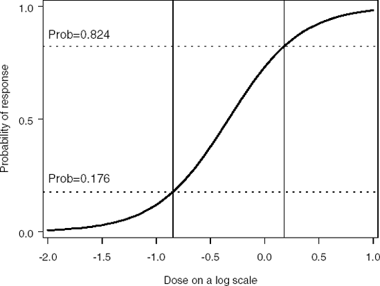
Dose-response models arise in clinical trials, either with a binary outcome (e.g., success-failure or dead-alive in toxicology studies; see Section 7.2) or continuous response (e.g., studies of pain medications when patients mark their pain level on a visual analog scale, see Section 7.4). In these examples, x represents the dose of a drug administered to the patient. Figure 7.1 illustrates the dependence of the probability of the success π(x) at the dose x for a two-parameter logistic model. Dotted horizontal lines correspond to the probabilities of success for the two optimal doses x₁^* and x₂^*. See Section 7.2 for details.

7.1.1.2. Bioassay studies

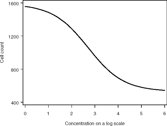
Multi-parameter logistic models, sometimes referred to as the E_max or Hill models, are widely used in bioassay studies. Examples include models that relate the concentration of an experimental drug to the percentage or number of surviving cells in cell-based assays or models that quantify the concentration of antigens or antibodies in enzyme-linked immunosorbent assays (ELISA). In this context, the design variable x represents the drug concentration level; see Sections 7.2 and 7.3 for details.

As an illustration, Figure 7.2 plots a four-parameter logistic model that describes the number of surviving bad cells in a cell-based assay versus drug concentration x on the log-scale. The concentration-effect relationship is negative. This is expected since an increase in the drug concentration usually reduces the number of cells.

7.1.1.3. Two-drug combination studies

Section 7.6.3 discusses two-drug combination studies in which two drugs (e.g., Drug A and Drug B) are administered simultaneously and their effect on the patient's outcome is analyzed. In this case, the design variable x is two-dimensional, i.e., x = (x₁,x₂), where x₁ is the dose of Drug A and x₂ is the dose of Drug B.

7.1.1.4. Clinical Pharmacokinetic Studies

Multiple blood samples are taken in virtually all clinical pharmacokinetic (PK) studies and the collected data are analyzed by means of various PK compartmental models. This analysis leads to quite sophisticated nonlinear mixed effects models which are discussed in Section 7.8. In these models x is a k-dimensional vector that represents a collection (sequence) of sampling times for a particular patient.

7.1.1.5. Cost-Based Designs

In the previous example (PK studies) it is quite obvious that each extra sample provides additional information. On the other hand, the number of samples that may be drawn from each patient is restricted because of blood volume limitations and other logistic and ethical reasons. Moreover, the analysis of each sample is associated with monetary cost. Thus, it makes sense to incorporate costs in the design. One potential approaches for the construction of cost-based designs is discussed in Section 7.9.

7.1.1.6. SAS Code and Data Sets

To save space, some SAS code has been shortened and some output is not shown. The complete SAS code and data sets used in this book are available on the book's companion web site at http://support.sas.com/publishing/bbu/companion_site/60622.html

7.1.2. Information Matrix, Maximum Likelihood Estimates and Optimality Criteria

For any parametric model, one of the main goals is to obtain the most precise estimates of unknown parameters θ. For example, in the context of a dose-response study, if clinical researchers can select doses x_i, in some admissible range, and number of patients n_i on each dose, then, given the total number of observations N, the question is how to allocate those doses and patients to obtain the best estimates of unknown parameters. The quality of estimators is traditionally measured by their variance-covariance matrix.

To introduce the theory underlying optimal design of experiments, we will assume that n_i is the number of independent observations y_ij that are made at design point x_i and N = n₁ + n₂ + ...+ n_n is the total number of observations, j = 1,..., n_i, i = 1,...., n. Let the probability density function of y_ij be p(y_ij|x_i,θ). For example, in the context of dose-response study, x_i is the ith dose of the drug and y_ij is the response of the jth patient on dose x_i.

Most of the examples discussed in this chapter deal with the case of a single measurement per patient, i.e., both x_i and y_ij are scalars (single dose and single response) and y_ij and y_i1,_j1 are independent if i ≠ i₁ or j ≠ j₁. The exceptions are Section 7.7 (two binary responses for the same patient, such as efficacy and toxicity, at a given dose x_i) and Sections 7.8 and 7.9 that consider the problem of designing experiments with multiple PK samples over time for the same patient, i.e., a design point is a sequence x_i = (x¹_i,x_i²,...,x_i^k) of k sampling times and y_ij = (y_ij¹,...,y_ij^k) is a vector of k observations. Note that in the latter case the elements of vector y_ij are, in general, correlated because they correspond to measurements on the same patient. However, similar to the case of a single measurement per patient, y_ij and y_i1,j₁ are still independent if i ≠ i₁ or j ≠ j₁.

7.1.2.1. Information Matrix

Let μ(x,θ) be an m × m information matrix of a single observation at point x,

where the expectation is taken with respect to the distribution of Y. The Fisher information matrix of the N experiments can be written as

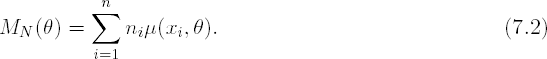
Further, let M(ξ,θ) be a normalized information matrix,

The collection ξ = {x_i,w_i} is called a normalized (continuous, or approximate) design with w₁ + ... + w_n = 1. In this setting N may be viewed as a resource available to researchers; see Section 7.9 for a different normalization.

7.1.2.2. Maximum Likelihood Estimates

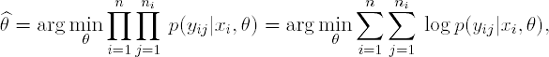
The maximum likelihood estimate (MLE) of θ is given by

It is well known that the variance-covariance matrix of for large samples is approximated by

where D(ξ,θ) = M⁻¹(ξ,θ) is the normalized variance-covariance matrix (Rao, 1973, Chapter 5). Throughout this chapter we assume that the normalized information matrix M(ξ,θ) is not singular and thus its inverse exists.

7.1.2.3. Optimality Criteria

In the convex design theory, it is standard to minimize various functionals depending on D(ξ,θ),

where Ψ is a selected functional (criterion of optimality). The optimization is performed with respect to designs ξ,

where χ is a design region, e.g., admissible doses in a dose-response study, and the weights, w₁,...,w_n, are continuous variables. The use of continuous weights leads to the concept of approximate optimal designs; the word approximate should draw attention to the fact that the solution of (7.5) does not generally give integer values n_i = N_wi. However, this solution is often acceptable, in particular when the total number of observations N is relatively large and we round n_i = N_wi to the nearest integer while keeping n₁ +...+ n_n = N (Pukelsheim, 1993).

The following optimality criteria are among the most popular ones:

D-optimality. Ψ = ln|D(ξ,θ)|, where |D| denotes the determinant of D.This criterion is often called a generalized variance criterion since the volume of the confidence ellipsoid for θ is proportional to |D(ξ,θ)|^1/2; see Fedorov and Hackl (1997, Chapter 2).

A-optimality. Ψ = tr[A D(ξ,θ)], where A is an m × m non-negative definite matrix (utility matrix) and tr(D) denotes the trace, or sum of diagonal elements, of D. For example, if A = m⁻¹I_m, where I_m is an m × m identity matrix, the A-criterion is based on the average variance of the parameter estimates:

c-optimality. Ψ = c^T D(ξ,θ)c, where c is an m-dimensional vector. A c-optimal design minimizes the variance of a linear combination of the model parameters, i.e., c^Tθ.

E-optimality. Ψ = λ_min[M(ξ,θ)] = λ_max[D(ξ,θ)], where λ_min(M) and λ_max(M) are minimal and maximal eigenvalues of M, respectively. Note that the length of the largest principal axis of the confidence ellipsoid is λ_min^−1/2[M(ξ,θ)].

I-optimality. Ψ = ∫χtr[μ(x,θ) D(ξ,θ)]dx. In linear regression models, tr[μ(x,θ)D(ξ,θ)] represents the variance of the predicted response.

Minimax optimality. Ψ = max_x∈χ tr[μ(x,θ) D(ξ,θ)].

For other criteria of optimality, see Fedorov (1972), Silvey (1980), or Pukelsheim (1993). It is important to note that the D-, A-, and E-optimality criteria may be ordered for any design since

see Fedorov and Hackl (1997, Chapter 2). Also, the disadvantage of c-optimal designs is that they are often singular, i.e., the corresponding variance-covariance matrix is degenerate.

7.1.2.4. D-Optimality Criterion

In this chapter we concentrate on the D-optimality criterion (note that the SAS programs described in this chapter can also be used to construct A-optimal designs). D-optimal designs are popular among theoretical and applied researchers due to the following considerations:

• D-optimal designs minimize the volume of the asymptotic confidence region for θ. This property is easy to explain to practitioners in various fields.

• D-optimal designs are invariant with respect to non-degenerate transformations of parameters (e.g., changes of the parameter scale).

• D-optimal designs are attractive in practice because they often perform well according to other optimality criteria; see Atkinson and Donev (1992, Chapter 11) or Fedorov and Hackl (1997).

7.1.3. Locally Optimal Designs

It is easy to see from the definition of the information matrix M(ξ,θ) that, in general, optimal designs depend on the unknown parameter vector θ. This assumption leads to the concept of locally optimal designs that are defined as follows: first we needs to specify a preliminary estimate of θ, e.g., , and then solve the optimization problem for the given (Chernoff, 1953, Fedorov, 1972).

It is worth noting that in linear parametric models the information matrix does not depend on θ which greatly simplifies the problem of computing optimal designs. Consider, for example, a linear regression model

with normally distributed residuals, i.e., ε_ij ∼ N(0,σ²(x_i)). Here f(x) = [f₁(x),..., f_m(x)]^T is a vector of pre-defined basis functions. The information matrix is given by (Fedorov and Hackl, 1997)

and thus one can construct designs that will be optimal for any value of θ. In non-linear models, one needs to select a value of θ first; however, once this value is fixed, the construction of an optimal design is absolutely the same as for linear problems.

Obviously, the quality of locally optimal designs may be poor if the preliminary estimate significantly differs from the true value of θ. We mention in passing that this problem can be tackled by using various techniques which include minimax designs (Fedorov and Hackl, 1997), Bayesian designs (Chaloner and Verdinelli, 1995), adaptive designs (Box and Hunter, 1965; Fedorov, 1972, Chapter 4; Zacks, 1996, Fedorov and Leonov, 2005, Section 5.6). While minimax and Bayesian approaches take into account prior uncertainties, they lead to optimization problems which are computationally more demanding than the construction of locally optimal designs. Instead of preliminary estimates of unknown parameters, we must provide an uncertainty set for the minimax approach and a prior distribution for Bayesian designs. The latter task is often based on a subjective judgement. Locally optimal designs serve as a reference point for other candidate designs, and sensitivity analysis with respect to parameter values is always required to validate the properties of a particular optimal design; see a discussion in Section 7.3.1.

In this chapter we concentrate on the construction of locally optimal designs.

7.1.4. Equivalence Theorem

Many theoretical results and numerical algorithms of the optimal experimental design theory rely on the following important theorem (Kiefer and Wolfowitz, 1960; Fedorov, 1972, White, 1973):

Generalized equivalence theorem.

A design ξ^* is locally D-optimal if and only if

where m is the number of model parameters. Similarly, a design ξ^* is locally A-optimal if and only if

The equality in (7.6) and (7.7) is attained at the support points of the optimal design ξ^*.

The ψ(x,ξ,θ) function is termed the sensitivity function of the corresponding criterion. The sensitivity function helps identify design points that provide the most information with respect to the chosen optimality criterion (Fedorov and Hackl, 1997, Section 2.4). For instance, if we consider dose-response studies, optimal designs can be constructed iteratively by choosing doses x^* that maximize the sensitivity function ψ(x,ξ,θ) over the admissible range of doses.

As shown in the next subsection, the general formulas (7.6) and (7.7) form a basis of numerical procedures for constructing D- and A-optimal designs.

7.1.5. Computation of Optimal Designs

Any numerical procedure for constructing optimal designs requires two key elements:

• The information matrix μ(x,θ) or, equivalently, sensitivity function ψ(x,ξ,θ).

• The design region χ (the set of admissible design points).

In all examples discussed in this chapter (except for the examples considered in Sections 7.8 and 7.9), we define the design region as a compact set, but search for optimal points on a pre-defined discrete grid. This grid can be rather fine in order to guarantee that the resulting design is close to the optimal one.

The main idea behind the general nonlinear design algorithm is that, at each step of the algorithm, the sensitivity function ψ(x,ξ,θ) is maximized over the design region to determine the best new support point (forward step) and then minimized over the support points of the current design to remove the worst point in the current design (backward step). See Fedorov and Hackl (1997) or Atkinson and Donev (1992) for details.

To define a design algorithm, let ξ_s = {X_is,w_is}, i = 1,...,n_s, be the design at Step s. Here {X_is} is the vector of support points in the current design and w_is is the vector of weights assigned to X_is. The iterative algorithm is of the following form:

where ξ(X) is a one-point design supported on point X.

Forward step.

At Step s, a point X⁺_s that maximizes ψ(x,ξ,θ) over x ∈ χ is added to the design ξ_s with weight α_s = γ_s, where γ_s = 1/(n₀ + s) and n₀ is the number of points in the initial design.

Backward step.

After that a point X⁻_s that minimizes ψ(x,ξ,θ) over all support points in the current design is deleted from the design with weight

In general, the user can change γ_s to c₁/(n₀ + c₂s), where c₁ and c₂ are two constant. The default values of the constants are c₁ = c₂ = 1.

In Section 7.2 we provide a detailed description of a SAS macro that implements the described optimal design algorithm for quantal dose-response models. However, once the information matrix μ(x,θ) or sensitivity function ψ(x,ξ,θ) are specified, the same technique can be used to generate optimal designs for any other model.

7.1.6. Existing Software

Computer algorithms for generating optimal designs have existed for quite some time (Fedorov, 1972; Wynn, 1970). These algorithms have been implemented in many commercially available software systems. Additionally, software written by academic groups is available. In general, the commercially available systems implement methods for problems such as simple linear regression and factorial designs, but not for more complex models such as nonlinear regression, beta regression, or population pharmacokinetics. Academic groups have developed and made available programs for the latter cases.

On the commercial side, SAS offers both SAS/QC (the OPTEX procedure) and JMP. The OPTEX procedure supports A- and D-optimal designs for simple regression models. JMP generates D-optimal factorial designs, as do software packages such as Statistica. In pharmacokinetic applications, the ADAPT II program developed at the University of Southern California implements c- and D-optimal and partially optimal design generation for individual pharmacokinetic models; however it does not support more complex population pharmacokinetic models (D'Argenio and Schumitzky, 1997). Ogungbenro et al (2005) implemented in Matlab the classical exchange algorithm for population PK experiments using D-optimality (note that the exchange algorithm improves the initial design with respect to selected optimality criterion, but, in general, does not converge to the optimal design).Retout and Mentré (2003) developed extensive implementation of population pharmacokinetic designs in S-Plus.

In this chapter we discuss SAS/IML implementation of the general algorithm (which cannot be executed in PROC OPTEX) with applications to several widely used nonlinear models. We also describe optimal design algorithms for population pharmacokinetic models analogous to the S-Plus programs of Retout and Mentré (2003).

7.1.7. Structure of SAS Programs

There are five components in the programs:

• inputs

• establishment of the design region

• calculation of the information matrix

• using the optimal design algorithm

• outputs.

Only the optimal design algorithm component is unchanged for any model; the other components are model-specific and need to be modified accordingly. In any model, calculation of the information matrix, is the critical (and most computationally intensive) step.