
12.8. Sensitivity Analysis
Sensitivity to model assumptions has been reported for about two decades (Verbeke and Molenberghs, 2000; Molenberghs and Verbeke, 2005). In an attempt to formulate an answer to these concerns, a number of authors have proposed strategies to study sensitivity.
Broadly, we could define a sensitivity analysis as one in which several statistical models are considered simultaneously and/or where a statistical model is further scrutinized using specialized tools (such as diagnostic measures). This rather loose and very general definition encompasses a wide variety of useful approaches. The simplest procedure is to fit a selected number of (MNAR) models which are all deemed plausible or to fit one model in which a preferred (primary) analysis is supplemented with a number of variations. The extent to which conclusions (inferences) are stable across such ranges provides an indication about the belief that can be put into them. Variations to a basic model can be constructed in different ways. The most obvious strategy is to consider various dependencies of the missing data process on the outcomes and/or on covariates. Alternatively, the distributional assumptions of the models can be changed.
Several publications have proposed the use of global and local influence tools (Verbeke et al., 2001; Verbeke and Molenberghs, 2000; Molenberghs and Verbeke, 2005). An important question is this: To what exactly are the sources causing an MNAR model to provide evidence for MNAR against MAR? There is evidence enough for us to believe that a multitude of outlying aspects is responsible for an apparent MNAR mechanism (Jansen et al., 2005). But it is not necessarily believable that the (outlying) nature of the missingness mechanism in one or a few subjects is responsible for an apparent MNAR mechanism. The consequence of this is that local influence should be applied and interpreted with due caution.
Further, within the selection model framework, Baker, Rosenberger, and DerSimonian (1992) proposed a model for multivariate and longitudinal binary data, subject to nonmonotone missingness. Jansen et al (2003) extended this model to allow for (possibly continuous) covariates, and developed a local influence strategy.
Next, classical inference procedures account for the imprecision resulting from the stochastic component of the model. Less attention is devoted to the uncertainty arising from (unplanned) incompleteness in the data, even though the majority of clinical studies suffer from incomplete follow-up. Molenberghs et al (2001) acknowledge both the status of imprecision, due to (finite) random sampling, as well as ignorance, due to incompleteness. Further, both can be combined into uncertainty (Kenward, Molenberghs and Goetghebeur, 2001).
Another route for sensitivity analysis is to consider pattern-mixture models as a complement to selection models. A third framework consists of so-called shared parameter models, where random effects are employed to describe the relationship between the measurement and dropout processes (Wu and Carroll, 1988; DeGruttola and Tu, 1994).
More detail on some of these procedures can be found in Molenberghs and Verbeke (2005). Let us now turn to the case of sensitivity analysis tools for selection models.
12.8.1.
12.8.1.1. Sensitivity Analysis for Selection Models
Particularly within the selection modeling framework, there has been an increasing literature on MNAR missingness. At the same time, concern has been growing precisely about the fact that models often rest on strong assumptions and relatively little evidence from the data themselves.
A sensible compromise between blindly shifting to MNAR models or ignoring them altogether, is to make them a component of a sensitivity analysis. In any case, fitting an MNAR dropout model should be subject to careful scrutiny. The modeler needs to pay attention, not only to the assumed distributional form of the model (Little, 1994b; Kenward, 1998), but also on the impact one or a few influential subjects may have on the dropout and/or measurement model parameters. Because fitting an MNAR dropout model is feasible by virtue of strong assumptions, such models are likely to pick up a wide variety of influences in the parameters describing the nonrandom part of the dropout mechanism. Hence, a good level of caution is in place.
First, an informal sensitivity analysis is applied on the Mastitis data. Next, the model of Diggle and Kenward (1994) is adapted to a form useful for sensitivity analysis, whereafter such a sensitivity analysis method, based on local influence (Cook, 1986; Thijs, Molenberghs and Verbeke, 2000), is introduced and applied to the Mastitis data.
12.8.1.2. Informal Sensitivity Analysis of the Mastitis Data
Diggle and Kenward (1994) and Kenward (1998) performed several analyses of the mastitis data described in Section 12.2. In Diggle and Kenward (1994), a separate mean for each group defined by the year of first lactation and a common time effect was considered, together with an unstructured 2 × 2 covariance matrix. The dropout model included both Yi1 and Yi2 and was reparameterized in terms of the size variable (Yi1 + Yi2)/2 and the increment Yi2 − Yi1. Kenward (1998) carried out what we could term a data-driven sensitivity analysis. The right panel of Figure 12.3 reveals that there appear to be two cows, #4 and #5 (black dots), with unusually large increments. Kenward conjectured that this might mean that these animals were ill during the first lactation year, producing an unusually low yield, whereas a normal yield was obtained during the second year. A simple multivariate Gaussian linear model is used to represent the marginal milk yield in the two years (i.e., the yield that would be, or was, observed in the absence of mastitis):
Note that β1 represents the change in average yield between the two years. The probability of mastitis is assumed to follow the logistic regression model:
The combined response/dropout model was fitted to the milk yields by using a program analogous to Program 12.7, presented in Section 12.7. In addition, the MAR model (ψ2 = 0) was fitted in the same way. These fits produced the parameter estimates displayed in the all column of Table 12.8.
Using the likelihoods to compare the fit of the two models, we get a difference G2 = 3.12. The corresponding tail probability from the X21 is 0.07. This test essentially examines the contribution of ψ2 to the fit of the model. Using the Wald statistic for the same purpose, gives a statistic of (−2.52)2/0.86 = 7.38, with corresponding X21 probability of 0.007. The discrepancy between the results of the two tests suggests that the asymptotic approximations on which these tests are based are not very accurate in this setting, and the standard error probability underestimates the true variability of the estimate of ψ2.
| MAR Dropout | |||
|---|---|---|---|
| Parameter | All | (7,53,54,66,69,70) | (4,5) |
| β0 | 5.77 (0.09) | 5.65 (0.09) | 5.81 (0.09) |
| β1 | 0.71 (0.11) | 0.67 (0.10) | 0.64 (0.09) |
| σ21 | 0.87 (0.12) | 0.72 (0.10) | 0.77 (0.11) |
| σ12 | 0.63 (0.13) | 0.44 (0.10) | 0.72 (0.13) |
| σ22 | 1.31 (0.20) | 1.00 (0.16) | 1.29 (0.20) |
| ψ0 | −3.33 (1.52) | −4.03 (1.76) | −3.09 (1.57) |
| ψ1 | 0.38 (0.25) | 0.50 (0.30) | 0.34 (0.26) |
| ψ2 | 0 | 0 | 0 |
| −2l | 624.13 | 552.24 | 574.19 |
| MNAR Dropout | |||
| Parameter | All | (7,53,54,66,69,70) | (4,5) |
| β0 | 5.77 (0.09) | 5.65 (0.09) | 5.81 (0.09) |
| β1 | 0.32 (0.14) | 0.36 (0.15) | 0.64 (0.14) |
| σ21 | 0.87 (0.12) | 0.72 (0.10) | 0.77 (0.11) |
| σ12 | 0.55 (0.13) | 0.38 (0.11) | 0.72 (0.13) |
| σ22 | 1.57 (0.28) | 1.16 (0.23) | 1.29 (0.20) |
| ψ0 | −0.34 (2.33) | −0.55 (2.57) | −3.10 (1.74) |
| ψ1 | 2.36 (0.79) | 2.01 (0.82) | 0.32 (0.72) |
| ψ2 | −2.52 (0.86) | −2.09 (0.98) | 0.01 (0.72) |
| −2l | 624.13 | 551.54 | 574.19 |
| G2 for MNAR | 3.12 | 0.70 | 0.0004 |
The dropout model estimated from the MNAR setting is as follows:
Some insight into this fitted model can be obtained by rewriting it in terms of the milk yield totals (Y1 + Y2) and increments (Y2 − Y1):
The probability of mastitis increases with larger negative increments, i.e., animals that showed (or would have shown) a greater decrease in yield over the two years have a higher probability of getting mastitis. The other differences in parameter estimates between the two models are consistent with this: the MNAR dropout model predicts a smaller average increment in yield (β1), with larger second year variance and smaller correlation caused by greater negative imputed differences between yields.
12.8.2. Local Influence
The local influence approach, suggested by Cook (1986), can be used to investigate the effect of extending an MAR model for dropout in the direction of MNAR dropout (Verbeke et al., 2001).
Again we consider the Diggle and Kenward (1994) model described in Section 12.7.1 for continuous longitudinal data subject to dropout. Since no data would be observed otherwise, we assume that the first measurement Yi1 is obtained for every subject in the study. We denote the probability of dropout at occasion k, given the subject was still in the study up to occasion k by g(hik,yik). For the dropout process, we now consider an extension of model (12.7.16), which can be written as
in which hik is the vector containing the history Hik as well as covariates. When ω equals zero and the model assumptions made are correct, the dropout model is MAR, and all parameters can be estimated using standard software since the measurement and dropout model can then be fitted separately. If ω ≠ 0, the dropout process is assumed to be MNAR. Now, a dropout model may be found to be MNAR solely because one or a few influential subjects have driven the analysis. To investigate sensitivity of estimation of quantities of interest, such as treatment effect, growth parameters, or the dropout model parameters, with respect to assumptions about the dropout model, we consider the following perturbed version of (12.8.21):
There is a fundamental difference with model (12.8.21) since the ωi should not be viewed as parameters: they are local, individual-specific perturbations around a null model. In our case, the null model will be the MAR model, corresponding to setting ω = 0 in (12.8.21). Thus the ωi are perturbations that will be used only to derive influence measures (Cook, 1986).
This scheme enables studying the effect of how small perturbation in the MNAR direction can have a large impact on key features of the model. Practically, one way of doing this is to construct local influence measures (Cook, 1986). Clearly, not all possible forms of impact resulting from sensitivity to dropout model assumptions will be found in this way, and the method proposed here should be viewed as one component of a sensitivity analysis (e.g. Molenberghs, Kenward, and Goetghebeur, 2001).
When small perturbations in a specific ωi lead to relatively large differences in the model parameters, it suggests that the subject is likely to drive the conclusions.
Cook (1986) suggests that more confidence can be put in a model which is relatively stable under small modifications. The best known perturbation schemes are based on case deletion (Cook and Weisberg 1982) in which the study of interest is the effect of completely removing cases from the analysis. A quite different paradigm is the local influence approach where the investigation concentrates on how the results of an analysis are changed under small perturbations of the model. In the framework of the linear mixed model Beckman, Nachtsheim and Cook (1987) used local influence to assess the effect of perturbing the error variances, the random-effects variances and the response vector. In the same context, Lesaffre and Verbeke (1998) have shown that the local influence approach is also useful for the detection of influential subjects in a longitudinal data analysis. Moreover, since the resulting influence diagnostics can be expressed analytically, they often can be decomposed in interpretable components, which yield additional insights in the reasons why some subjects are more influential than others.
We are interested in the influence of MNAR dropout on the parameters of interest. This can be done in a meaningful way by considering (12.8.22) as the dropout model. Indeed, ωi = 0 for all i corresponds to an MAR process, which cannot influence the measurement model parameters. When small perturbations in a specific ωi lead to relatively large differences in the model parameters, then this suggests that these subjects may have a large impact on the final analysis. However, even though we may be tempted to conclude that such subjects drop out non-randomly, this conclusion is misguided since we are not aiming to detect (groups of) subjects that drop out non-randomly but rather subjects that have a considerable impact on the dropout and measurement model parameters. Indeed, a key observation is that a subject that drives the conclusions towards MNAR may be doing so, not only because its true data generating mechanism is of an MNAR type, but also for a wide variety of other reasons, such as an unusual mean profile or autocorrelation structure. Earlier analyses have shown that this may indeed be the case. Likewise, it is possible that subjects, deviating from the bulk of the data because they are generated under MNAR, go undetected by this technique. This reinforces the concept thet we must reflect carefully upon which anomalous features are typically detected and which ones typically go unnoticed.
12.8.2.1. Key Concepts
Let us now introduce the key concepts of local influence. We denote the log-likelihood function corresponding to model (12.8.22) by

in which li (γ|ωi) is the contribution of the ith individual to the log-likelihood, and where γ = (θ,ψ) is the s-dimensional vector, grouping the parameters of the measurement model and the dropout model, not including the N × 1 vector ω = (ω1, ω2, ..., ωN)′ of weights defining the perturbation of the MAR model. It is assumed that ω belongs to an open subset Ω of IRN. For ω equal to ω0 = (0, 0,..., 0)′, l(γ|ω0) is the log-likelihood function which corresponds to a MAR dropout model.
Let ![]() be the maximum likelihood estimator for γ, obtained by maximizing l(γ|ω0), and let
be the maximum likelihood estimator for γ, obtained by maximizing l(γ|ω0), and let ![]() w denote the maximum likelihood estimator for γ under l (γ|ω). The local influence approach now compares
w denote the maximum likelihood estimator for γ under l (γ|ω). The local influence approach now compares ![]() w with
w with ![]() . Similar estimates indicate that the parameter estimates are robust with respect to perturbations of the MAR model in the direction of non-random dropout. Strongly different estimates suggest that the estimation procedure is highly sensitive to such perturbations, which suggests that the choice between an MAR model and a non-random dropout model highly affects the results of the analysis. Cook (1986) proposed to measure the distance between
. Similar estimates indicate that the parameter estimates are robust with respect to perturbations of the MAR model in the direction of non-random dropout. Strongly different estimates suggest that the estimation procedure is highly sensitive to such perturbations, which suggests that the choice between an MAR model and a non-random dropout model highly affects the results of the analysis. Cook (1986) proposed to measure the distance between ![]() w and
w and ![]() by the so-called likelihood displacement, defined by
by the so-called likelihood displacement, defined by
This takes into account the variability of ![]() . Indeed, LD(ω) will be large if l(γ|ω0) is strongly curved at
. Indeed, LD(ω) will be large if l(γ|ω0) is strongly curved at ![]() , which means that γ is estimated with high precision, and small otherwise. Therefore, a graph of LD(ω) versus ω contains essential information on the influence of perturbations. It is useful to view this graph as the geometric surface formed by the values of the N + 1 dimensional vector ξ(ω) = (ω′, LD(ω))′ as ω varies throughout Ω.
, which means that γ is estimated with high precision, and small otherwise. Therefore, a graph of LD(ω) versus ω contains essential information on the influence of perturbations. It is useful to view this graph as the geometric surface formed by the values of the N + 1 dimensional vector ξ(ω) = (ω′, LD(ω))′ as ω varies throughout Ω.
Since this influence graph can only be depicted when N = 2, Cook (1986) proposed to look at local influence, i.e., at the normal curvatures Ch of ξ(ω) in ω0, in the direction of some N dimensional vector h of unit length. Let Δi be the s dimensional vector defined by

and define Δ as the (s × N) matrix with Δi as its ith column. Further, let ![]() denote the (s × s) matrix of second order derivatives of l(γ|ω0) with respect to γ, also evaluated at γ =
denote the (s × s) matrix of second order derivatives of l(γ|ω0) with respect to γ, also evaluated at γ = ![]() . Cook (1986) has then shown that Ch can be easily calculated by
. Cook (1986) has then shown that Ch can be easily calculated by
Obviously, Ch can be calculated for any direction h. One evident choice is the vector hi containing one in the ith position and zero elsewhere, corresponding to the perturbation of the ith weight only. This reflects the influence of allowing the ith subject to drop out non-randomly, while the others can only drop out at random. The corresponding local influence measure, denoted by Ci, then becomes Ci = 2|Δi′![]() −1Δi|. Another important direction is the direction hmax of maximal normal curvature Cmax. It shows how to perturb the MAR model to obtain the largest local changes in the likelihood displacement. It is readily seen that Cmax is the largest eigenvalue of −2 Δ′
−1Δi|. Another important direction is the direction hmax of maximal normal curvature Cmax. It shows how to perturb the MAR model to obtain the largest local changes in the likelihood displacement. It is readily seen that Cmax is the largest eigenvalue of −2 Δ′![]() −1Δ, and that hmax is the corresponding eigenvector.
−1Δ, and that hmax is the corresponding eigenvector.
12.8.2.2. Local Influence in the Diggle-Kenward Model
As discussed in the previous section, calculation of local influence measures merely reduces to evaluation of Δ and ![]() . Expressions for the elements of
. Expressions for the elements of ![]() in case Σi = σ2
I are given by Lesaffre and Verbeke (1998), and can easily be extended to the more general case considered here. Further, it can be shown that the components of the columns Δi of Δ are given by
in case Σi = σ2
I are given by Lesaffre and Verbeke (1998), and can easily be extended to the more general case considered here. Further, it can be shown that the components of the columns Δi of Δ are given by
for complete sequences (no dropout) and by
for incomplete sequences. All above expressions are evaluated at ![]() , and where g(hij) = g(hij, yij)|ωi = 0, is the MAR version of the dropout model.
, and where g(hij) = g(hij, yij)|ωi = 0, is the MAR version of the dropout model.
Let Vi,11 be the predicted covariance matrix for the observed vector (yi1, ..., yi,d−1)′, Vi,22 is the predicted variance for the missing observation yid, and Vi,12 is the vector of predicted covariances between the elements of the observed vector and the missing observation. It then follows from the linear mixed model (12.7.15) that the conditional expectation for the observation at dropout, given the history, equals
which is used in (12.8.24).
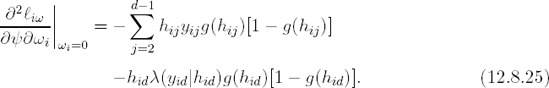
The derivatives of (12.8.26) with respect to the measurement model parameters are
where xid′ is the dth row of Xi, and where Xi,(d−1) indicates the first (d − 1) rows Xi. Further, α indicates the subvector of covariance parameters within the vector θ.
In practice, the parameter θ in the measurement model is often of primary interest. Since ![]() is block-diagonal with blocks
is block-diagonal with blocks ![]() (θ) and
(θ) and ![]() (ψ), we can write for any unit vector h, Ch = Ch(θ) + Ch(ψ). It now immediately follows from (12.8.24) that influence on θ only arises from those measurement occasions at which dropout occurs. In particular, from expression (12.8.24), it is clear that the corresponding contribution is large only if (1) the dropout probability is small but the subject disappears nevertheless and (2) the conditional mean strongly depends on the parameter of interest. This implies that complete sequences cannot be influential in the strict sense (Ci(θ) = 0) and that incomplete sequences only contribute at the actual dropout time.
(ψ), we can write for any unit vector h, Ch = Ch(θ) + Ch(ψ). It now immediately follows from (12.8.24) that influence on θ only arises from those measurement occasions at which dropout occurs. In particular, from expression (12.8.24), it is clear that the corresponding contribution is large only if (1) the dropout probability is small but the subject disappears nevertheless and (2) the conditional mean strongly depends on the parameter of interest. This implies that complete sequences cannot be influential in the strict sense (Ci(θ) = 0) and that incomplete sequences only contribute at the actual dropout time.
12.8.2.3. Implementation of Local Influence Analysis in SAS
Program 12.8 relies on SAS/IML to calculate the normal curvature Ch of ξ(ω) in ω0, in the direction the unit vector h.
As in Program 12.7, we first need to create the X and Z matrices, Y and INITIAL vectors and NSUB and NTIME parameters (this can be accomplished in PROC IML using in a program analogous to Program 12.6). The initial parameters should be the estimates of the parameters of the MAR model, fitted using a program analogous to Program 12.7. Next, we need the INTEGR and LOGLIK modules introduced in Program 12.7. These are called to calculate the log-likelihood function of the Diggle and Kenward (1994) model under the MNAR assumption. This is needed for the evaluation of Δ as well as for ![]() . Program 12.8 also calls the DELTA module to calculate the Δ vector, whereas
. Program 12.8 also calls the DELTA module to calculate the Δ vector, whereas ![]() is calculated using the NLPFDD module of SAS/IML which was introduced earlier in Section 12.7.2. Finally, Program 12.8 created the C_MATRIX data set that contains the following normal curvatures in the direction of the unit vector hi containing one in the ith position and zero elsewhere,
is calculated using the NLPFDD module of SAS/IML which was introduced earlier in Section 12.7.2. Finally, Program 12.8 created the C_MATRIX data set that contains the following normal curvatures in the direction of the unit vector hi containing one in the ith position and zero elsewhere,
C = Ci, C1 = Ci(β), C2 = Ci(α), C12 = Ci(θ), C3 = Ch(ψ),
and the normal curvature in the direction of HMAX = hmax of maximal normal curvature CMAX = Cmax. The C_MATRIX data set can now be used to picture the local influence measures. The complete SAS code of Program 12.8 is provided on the book's companion Web site.
Example 12-8. Local influence sensitivity analysis
proc iml;
    use x; read all into x;
    use y; read all into y;
    use nsub; read all into nsub;
    use ntime; read all into ntime;
    use initial; read all into initial;
    g=j(nsub,1,0);
    start integr(yd) global(psi,ecurr,vcurr,lastobs);
    ...
    finish integr;
start loglik(parameters) global(lastobs,vcurr,ecurr,x,z,y,nsub,ntime,nrun,psi);
...
finish loglik;
start delta(parameters) global(lastobs,vcurr,ecurr,x,z,y,nsub,ntime,nrun,psi);
...
finish delta;
opt=j(1,11,0);
opt[1]=1;
opt[2]=5;
con={. . 0 . 0 . . ,
. . . . . . . };
call nlpnrr(rc,est,"loglik",initial,opt,con);
* Calculation of the Hessian;
...
* Calculation of the C-matrix;
...
create c_matrix var {subject ci c12i c3i c1i c2i hmax cmax};
append;
quit; |
12.8.2.4. Mastitis Data
We will apply the local influence method to the mastitis data described in Section 12.2. For the measurement process, we use model (12.8.19) and thus the covariance matrix Vi is unstructured. Since there are only two measurement occasions Yi1 and Yi2, the components of the columns Δi of Δ are given by (12.8.23), when both measurements are available, and by (12.8.24) and (12.8.25), when only the first measurement is taken. In the latter case, we need Vi,11, Vi,12, and their derivatives with respect to the three variance components σ21, σ12 and σ22, to calculate (12.8.26), (12.8.27), and (12.8.28). Since an incomplete sequence can only occur when the cow dropped out at the second measurement occasion, we have that Vi,11 = σ21 and Vi,12 = σ12, and thus
If we have another form of model (12.7.15), the program can be adapted, by changing Vi, Vi,11, Vi,12, and the derivatives.
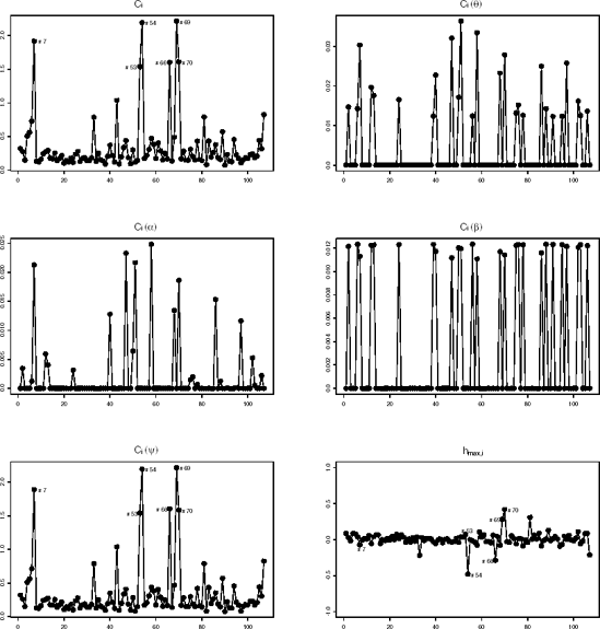
The results of the local influence analysis of the mastitis data (based on Program 12.8) are shown in Figure 12.7 which suggests that there are six influential subjects: #7, #53, #54, #66, #69, and #70, while #4 and #5 are not recovered. It is interesting to consider an analysis with these six cows removed. The influence on the likelihood ratio test is a little smaller then in the case of removing #4 and #5: G2 = 0.07 compared to G2 = 0.0004 when removing #4 and #5 instead of the original 3.12. The influence on the measurement model parameters under both random and non-random dropout is small for the fixed effects parameters, but not so small for the covariance components parameters.
12.8.2.5. Local and Global Influence
Let us now discuss differences between local and global influence. It is very important to realize that we should not expect agreement between the deletion and local influence analyses. The latter focuses on the sensitivity of the results with respect to the assumed dropout model, more specifically how the results change when the MAR model is extended into the direction of non-random dropout. In Ci(β) and Ci(α) panels, little or no influence is detected, certainly when the scale is compared to the one of Ci(ψ). This is obvious for subjects #53, #54, #66, and #69, since all these are complete and hence Ci(θ)≡ 0, placing all influence on Ci(ψ). Of course, a legitimate concern is precisely where we should place a cut-off between subjects that are influential and those that are not. Clearly, additional work studying the stochastic behavior of the influence measures would be helpful. Meanwhile, informal guidelines can be used, such as studying 5% of the relatively most influential subjects.
Figure 12-7. Index plots of Ci, Ci(θ), Ci(α), Ci(β), Ci(ψ) and of the components of the direction hmax,i of maximal curvature in the mastitis example
Kenward (1998) observed that Cows #4 and #5 in the mastitis example are unusual on the basis of their increment. This is in line with several other applications of similar dropout models (Molenberghs, Kenward and Lesaffre, 1997) where it was found that a strong incremental component apparently yields a non-random dropout model. From the analysis done, it is clear that such a conclusion may not be well founded, since removal of #4 and #5 leads to disappearance of the non-random component (see Table 12.8).