
11.4. Regression Modeling
In this section we will introduce statistical methods for addressing the second objective of dose-ranging studies, namely, characterization of the dose-response curve. While in the previous section we were concerned with hypothesis testing, this section will focus on modeling dose-response functions and estimation of their parameters. We will consider approaches based on linear and sigmoid (or Emax) models.
It is important to note that the modeling approaches discussed below can be used to study effects of either actual dose or pharmacokinetic exposure parameters (e.g., area under the time-plasma concentration curve or maximum plasma concentration) on the response variable of interest. When the drug's distribution follows simple pharmacokinetic models, e.g., a one-compartmental model with a first-order transfer rate, the exposure parameters are proportional to the dose (this is known as pharmacokinetic dose-proportionality). In this case, the two approaches yield similar results. However, in the presence of complex pharmacokinetics, dose-proportionality may not hold and exposure-response models are more informative than dose-response models.
11.4.1. Linear Models
Here we will consider a simple approach to modeling the dose- or exposure-response relationship in dose-ranging trials. This approach relies on linear models. Linear models often serve as a reasonable first approximation to an unknown dose-response function and can be justified in a variety of dose-ranging trials unless the underlying biological processes exhibit ceiling or plateau effects. If a linear model is deemed appropriate, it is easy to fit using PROC REG (parallel group designs) or PROC MIXED (parallel group or cross-over designs).
As an illustration, we will fit a linear model to approximate the relationship between the drug exposure (measured by the maximum plasma concentration of the study drug, Cmax) and mean fasting glucose level in the diabetes trial. Program 11.6 fits a linear repeated-measures model to the glucose and Cmax measurements in the Diabetes data set using PROC MIXED. A repeated-measures model specified by the REPEATED statement is used here to account for the cross-over nature of this trial. The program also computes predicted fasting glucose levels and a confidence band for the true exposure-response function. The predicted values and confidence intervals are requested using the OUTPREDM option in the MODEL statement.
Example 11-6. Linear exposure-response model in the diabetes trial
proc mixed data=diabetes;
    class subject;
    model glucose=cmax/outpredm=predict;
    repeated/type=un subject=subject;
proc sort data=predict;
    by cmax;
axis1 minor=none value=(color=black)
    label=(color=black angle=90 "Glucose level (mg/dL)')
    order=(100 to 200 by 20);
axis2 minor=none value=(color=black) label=(color=black "Cmax (ng/mL)'),
symbol1 value=none i=join color=black line=20;
symbol2 value=none i=join color=black line=1;
symbol3 value=none i=join color=black line=20;
symbol4 value=dot i=none color=black;
proc gplot data=predict;
    plot (lower pred upper glucose)*cmax/overlay frame haxis=axis2 vaxis=axis1;
    run;
quit; |
Example. Output from Program 11.6
Solution for Fixed Effects

                         Standard
Effect       Estimate       Error      DF    t Value    Pr > |t|

Intercept      175.78      2.1279      23      82.61      <.0001
cmax −0.03312 0.003048 23 −10.87 <.0001 |
Output 11.6 lists estimates of the intercept (INTERCEPT) and slope (CMAX) of the linear exposure-response model produced by PROC MIXED. The intercept represents the baseline (placebo) effect and the slope indicates the rate at which the mean glucose concentration decreases with increasing exposure.
Figure 11-4. Fasting glucose levels predicted by a linear model in the diabetes trial
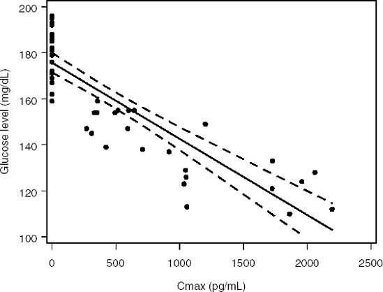
Figure 11.4 depicts the predicted fasting glucose concentration as a function of Cmax along with a series of 95% confidence intervals that form a confidence band. It is clear from Figure 11.4 that the linear model provides a fairly poor fit to the fasting glucose data. Most of the dots representing individual glucose measurements lie below the fitted line and outside the confidence band. The pattern of individual measurements suggests that the true exposure-response relationship is likely to be curvilinear.
11.4.2. Sigmoid Models
We saw in the previous subsection that linear models may not always provide an adequate approximation to exposure-response functions. Non-linear models perform better in practice and are generally more appealing from a clinical perspective. One way to improve the performance of simple linear models is by applying a non-linear transformation of the independent variable, e.g., fitting a linear model with a log-transformed AUC or Cmax. Another popular non-linear modeling approach relies on the sigmoid model (also referred to as the Emax model). This model describes the true treatment effect E as a sigmoid function of drug exposure d:
In this model,
E0 is the baseline effect at the zero exposure level.
Emax represents the maximum possible effect of the experimental drug on the response variable relative to baseline.
d50 is the exposure level at half-maximal effect (sometimes called the median effective dose). It is easy to verify that the treatment effect E is equal to E0 + Emax/2 when d = d50.
γ determines the steepness of the sigmoid function. The γ parameter, known as the Hill coefficient in the pharmacodynamic literature, typically ranges between 1 and 3.
In cross-over trials, the introduced sigmoid model needs to be modified to account for repeated measurements on the same subject. This is achieved by including a random subject term in the model. Program 11.7 uses a sigmoid model with a random subject term to approximate the exposure-response curve in the diabetes trial:
where η is a random subject term and the γ parameter is set to 1 to simplify non-linear modeling in this small data set. Note that E is a decreasing function of d since the experimental drug is expected to lower the glucose level. To fit this complex non-linear model, the program relies on the NLMIXED procedure, a powerful procedure that supports a broad class of non-linear models with random effects.
In Program 11.7, the response variable (GLUCOSE) is modeled as a non-linear function of a fixed exposure effect (CMAX) and a random subject effect (SUB). The subject effects are assumed to be normally distributed. The SUBJECT option in the RANDOM statement identifies groups of related observations made on the same individual.
The initial values of the baseline and maximum effects, E0 and Emax, as well as the median effective dose, d50, were taken from the dose-response function depicted in Figure 11.1. The initial values of both the within-subject (INTRASUBJECT) and between-subject (INTERSUBJECT) variances were 1.
Example 11-7. Sigmoid exposure-response model in the diabetes trial
proc nlmixed data=diabetes;
    ods select ParameterEstimates;
    parms e0=180 emax=60 d50=900 intrasigma=1 intersigma=1;
    prediction=e0-(sub+emax)*cmax/(cmax+d50);
    model glucose~normal(prediction,intersigma);
    random sub~normal(0,intrasigma) subject=subject;
    predict e0-emax*cmax/(cmax+d50) out=predict;
proc sort data=predict;
    by cmax;
axis1 minor=none value=(color=black)
    label=(color=black angle=90 "Glucose level (mg/dL)')
    order=(100 to 200 by 20);
axis2 minor=none value=(color=black) label=(color=black "Cmax (ng/mL)'),
symbol1 value=none i=join color=black line=20;
symbol2 value=none i=join color=black line=1;
symbol3 value=none i=join color=black line=20;
symbol4 value=dot i=none color=black;
proc gplot data=predict;
    plot (lower pred upper glucose)*cmax/
        overlay frame haxis=axis2 vaxis=axis1;
    run;
quit; |
Example. Output from Program 11.7
Parameter Estimates

                      Standard
Parameter   Estimate     Error    DF  t Value  Pr > |t|   Alpha

e0            179.36    2.0873    47    85.93    <.0001    0.05
emax         87.1425   16.3395    47     5.33    <.0001    0.05
d50           899.75    396.02    47     2.27    0.0277    0.05
intrasigma    3.0613    148.03    47     0.02    0.9836    0.05
intersigma    101.12   24.8511    47     4.07    0.0002    0.05
Parameter Estimates Parameter Lower Upper Gradient e0 175.16 183.56 0.000378 emax 54.2717 120.01 −0.00006 d50 103.05 1696.45 0.001309 intrasigma −294.73 300.85 0.003211 intersigma 51.1297 151.12 −0.00003 |
Output 11.6 shows estimates of the parameters of the sigmoid model. The estimated E0, Emax and d50 parameters are generally close to their initial values. According to the fitted sigmoid model, the experimental drug is theoretically capable of reducing the mean glucose level to 92 mg/dL (= 179 − 87). The half-maximal effect is achieved at the median effective dose (D50) which is equal to 900 mg/dL. The within-subject variance (INTRASUBJECT) is considerably smaller than the between-subject variance (INTERSUBJECT).
Figure 11-5. Fasting glucose levels (mg/dL) predicted by a sigmoid model in the diabetes trial
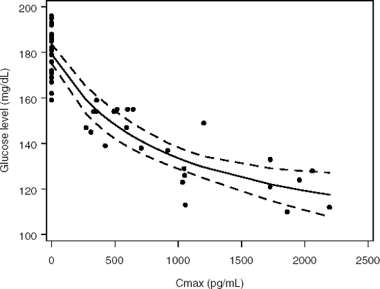
Figure 11.5 displays the fasting glucose concentration predicted by the sigmoid model with a 95% confidence band. The fitted dose-response curve has a concave shape and fits the data well. There is no obvious pattern in the residuals and many observations fall within the 95% confidence band around the fitted curve.
The fitted model can be used for an informal determination of doses or drug exposures to be investigated in Phase II trials (Ruberg, 1995b). Suppose, for example, that the objective of the diabetes trial was to reduce the glucose concentration to a "normal' level defined as 126 mg/dL. We can see from Figure 11.5 that the lower confidence limit is below this clinically important threshold when the maximum plasma concentration is greater than 1200 pg/mL. Secondly, the mean glucose concentration falls below the 126 mg/dL threshold around Cmax = 1700 pg/mL. Using this information, we could define the minimally effective exposure level as a value between 1200 and 1700 pg/mL and effective exposure levels as values exceeding 1700 pg/mL.