
6.2. Two Independent Sample Setting
An experiment involving two independent groups is one of the most elementary types of investigations in scientific research, yet is no less valuable than many other more complicated multifactor or multilevel experiments. Typically, subjects are randomly assigned to one of two groups, a treatment is applied, and a measurement is collected on all subjects in both groups. It is then usually the desire of the investigators to ascertain whether sufficient evidence exists to declare the two groups to be different. Although many are familiar enough with statistics to perform two sample comparisons, often, key assumptions are swept under the rug, as it were, and as a result, errors in inference sometimes occur.
This section will begin with a review of the assumptions necessary to perform a two-sample comparison and then discuss a common means to compare the location parameters of two groups (Section 6.2.2). Section 6.2.3 will discuss one possible solution for the problem of unequal spread (heteroscedasticity) between two groups. One important false notion about the rank transform and its effect on groups with unequal dispersion will also be discussed. This section will include examples of data from two clinical trials.
6.2.1. A Review of the Two-Sample Setting
We will begin this section with a slight bit of mathematical formality. Suppose that we have two random samples, denoted X1,...,Xn1 and Y1,...,Yn2. We assume that the X's and Y's come from a distribution, say, F. Typically, the two-sample problem is characterized by a desire to perform an inference about a shift in location between the distributions of the two samples. Suppose FX = F(μ) is the distribution of the X's (with location parameter μ) and FY = F(μ + δ) is the distribution of the Y's, shifted by δ. What can be said about a measure δ, where FX(μ) = FY(μ + δ)? Is δ "reasonably close" to zero or not? If the X's follow a Gaussian (normal) distribution, say, N(μ1,σ2), and the Y's are distributed from another Gaussian distribution, say, N(μ2,σ2), we could think of the problem as considering whether μ1 = μ2 + δ. In this classic "normal" case, it is very important to note that we assume that the variance of the two Gaussian distributions is "reasonably" the same (often referred to as a common σ2). If latter is not true, we are working under the conditions of a famous setting in statistics, the Behrens-Fisher problem, and we need to make some changes to our inferential procedures. In either case, some form of a Student's t-statistic may be used to compare the locations (means) of the two distributions.
Do the measurements we collect come from a Gaussian distribution? In drug discovery settings in the pharmaceutical industry, sample sizes in some investigations can be very small (total sample size for a study less than 12) and, thus, it might be very difficult to establish the form of a measurement's distribution. Moreover, as little is known in the discovery stages of research about the impact of a compound on a complicated mammalian physiology, a seemingly outlying or extreme value may in fact be part of the tail of a highly skewed distribution. With small sample sizes and limited background information, it really is anyone's best guess as to the parametric form of a measurement's distribution.
What if the distributions are not Gaussian? The standard Student's t-test will perform at the designated level of statistical significance. In most cases, departures from a Gaussian distribution do not greatly affect the operating characteristics of inferential procedures if the two distributions have mild skewness or kurtosis. However, moderate to high levels of skewness can influence the power of a comparison of two location parameters (Bickel and Docksum, 1977) and, thus, influence our ability to identify potentially efficacious or toxic compounds.
Shortly, we will look at an example of a two-sample setting where the data are sufficiently skewed to warrant the introduction of a distribution-free test that serves as a competitor to the standard Student's two-sample t-test. First, however, it is necessary to describe a setting where such data could be found: asthma treatment research.
EXAMPLE: Asthma Clinical Trial
Asthma is a disease characterized by an obstruction of airflow in the lungs, and thus referred to as an obstructive ventilatory defect (National Asthma Council Australia, 2002). One of the chief measurements used to characterize the degree of disease is the Forced Expiratory Volume in 1 second, or FEV1. A patient will exhale into a device (a spirometer) that will measure his or her volume of expired air.
Physicians working on developing new drugs for treatment of asthma are interested in a measure that characterizes the degree of reversibility of the airflow obstruction. Thus, a patient's baseline FEV1 will be measured before treatment (at baseline). Typically, 10–15 minutes after the administration of a treatment (e.g., a beta2 agonist bronchodilator), FEV1 will be measured a second time. The percent improvement in FEV1 from baseline is used to measure the effectiveness of a new drug:
A medically important improvement is typically at least 12%; however, not all researchers in the field accept this level.
Consider a simple trial to establish the efficacy of a new treatment for asthma. Seven hundred patients are randomized to one of two groups. Patients randomized to the first group had baseline FEV1 measurements collected, then received a placebo treatment and, at 10 minutes post-treatment, had a second FEV1 measurement taken. The procedure was similar for the second group of patients, except that after measurement at baseline, they received a novel treatment. The percent changes in FEV1 collected in this study are included in the SPIRO data set that can be found on the book's companion Web site. Table 6.1 provides a summary of the results in the two treatment groups and Figure 6.1 displays a box plot summary of percent changes in FEV1.
| Group | Sample size | Mean | Standard deviation | Median | Interquartile range |
|---|---|---|---|---|---|
| Placebo | 347 | 9.58 | 30.89 | 14.00 | 37.55 |
| Treated | 343 | 13.75 | 20.08 | 14.14 | 29.16 |
Figure 6-1. Results of the asthma clinical trial
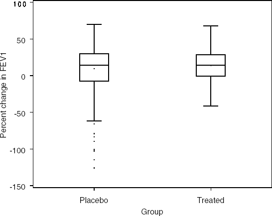
The box plots and summary statistics provide some interesting insight into the results of the study. First, it appears for a small number of patients (10 total) a full percent change score was unavailable. Also, it appears that the placebo group included some patients whose results were dramatically worse between the initial baseline FEV1 and the later post-treatment measurement (note the large number of outliers represented by dots outside the fence in the box plot). These results produce a long downward tail in the distribution of change from baseline values and contribute to skewing of the distribution. This also can be observed by the difference of 4 percentage points between the mean and median for this group. The level of dispersion, or spread, of the two groups is not identical; however, it is not greatly different. How do we compare the location parameters of two distributions in the presence of equal, or similar, dispersion?
6.2.2. Comparing the Location of Two Independent Samples I: Similar Dispersion
Returning to the notation introduced previously in Section 6.2.1:
Group 1: X1,...,Xn1 with Xi ~ F(μ), i = 1,...,n1.
Group 2: Y1,...,Yn2 with Yj ~ F(μ + δ), j = 1,...,n2.
Here F(λ) is a continuous distribution with location parameter, λ.
6.2.2.1. Wilcoxon Rank Sum Test
The inference of interest is H0 : δ = 0 versus HA : δ > 0. This null hypothesis can be tested using the Wilcoxon Rank Sum test (Wilcoxon, 1945). To carry out this test, we begin by performing a joint ranking of the X's and Y's from the smallest value to the largest. If two or more values are tied, their ranks are replaced by the average of the tied ranks. The Wilcoxon, W, is simply the sum of the corresponding ranks for the Y's, i.e., W = Σn2j=1 Rj, where Rj is the rank of Yj in the combined sample. We reject H0 : δ = 0 at an α level if W ≥ cα;, for a cutoff value, cα;, that corresponds to the null distribution of W.
If the minimum of n1 and n2 is sufficiently large, an approximate procedure may be employed. The Wilcoxon Rank Sum statistic specified above requires some modifications so that the Central Limit Theorem will hold and the statistic will be asymptotically normal:

What is the form of the variance of the W statistics for tied observations, i.e., Var(WT)? Suppose that for all n1 + n2 observations, tied groups of size tv (1,2,...,v,..., ξ) exist. The variance in the denominator of the statistic is as follows (Hollander and Wolfe, 1999):
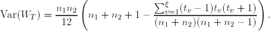
The large sample version of the one-sided hypothesis test is then: Reject H0 : δ = 0 at an α level if WL ≥ zα, where zα is the 100(1 − α) quantile from a standard normal distribution.
Before we embark on a discussion of the lower-tailed and two-sided Wilcoxon Rank Sum tests, let's return to the asthma clinical trial example. Program 6.1 uses the NPAR1WAY procedure to perform the Wilcoxon Rank Sum test using the SPIRO data set. The Wilcoxon Rank Sum test is requested by the WILCOXON option. PROC NPAR1WAY automatically uses tied ranks and performs the appropriate adjustment to the test statistic based upon the large sample form of the statistic. The ODS statement is included to select the relevant portion of the procedure's output. The CLASS statement identifies the classification or grouping variable. the VAR statement identifies the response variable (percent change in FEV1).
Example 6-1. Wilcoxon Rank Sum test in the asthma trial example
proc npar1way data=spiro wilcoxon;
    ods select WilcoxonTest;
    class group;
    var fevpc;
run; |
Example. Output from Program 6.1
Wilcoxon Two-Sample Test

                          Statistic             120620.0000

                          Normal Approximation
                          Z                          0.8071
                          One-Sided Pr >  Z          0.2098
                          Two-Sided Pr > |Z|         0.4196

                          t Approximation
                          One-Sided Pr >  Z          0.2099
                          Two-Sided Pr > |Z|         0.4199

Z includes a continuity correction of 0.5. |
We conclude from Output 6.1 that a statistically significant improvement from baseline FEV1 did not exist at the 0.05 level of statistical significance (one-tailed p-value based on the normal approximation is 0.2098).
6.2.2.2. Student's two-sample t-test
What about other methods of data analysis? Commonly, in the face of skewed data, analysts will use some form of transformation. A commonly used transformation is the natural logarithm transformation applied to each of the responses. In the example illustrated previously, a log or power transformation will not work, as negative values exist in the data. Suppose we chose to ignore the long tail of the placebo group's distribution and performed a standard Student's two-sample t-test (Student, 1908). Program 6.2 performs Student's two-sample t-test using PROC TTEST. The code to perform a Student's two-sample t-test is very similar to the PROC NPAR1WAY code. As in Program 6.1, the ODS statement is included to select the relevant portion of the procedure's output.
Example 6-2. Student's two-sample t-test in the asthma trial example
proc ttest data=spiro;
    ods select ttests;
    class group;
    var fevpc;
run; |
Example. Output from Program 6.2
T-Tests

        Variable    Method           Variances      DF    t Value    Pr > |t|

        fevpc       Pooled           Equal         688      −2.10      0.0363
fevpc Satterthwaite Unequal 595 −2.10 0.0360 |
If we select the two-tailed p-value from Output 6.2 (assuming unequal variances in the two groups) and adjust it so that it reflects a one-tailed t-test in (p = 0.036/2 = 0.018), we will infer that the mean FEV1 percent change score was statistically significantly increased by the new treatment. The long tail of extreme low responses in the control group influenced this conclusion. The extreme negative FEV1 percent change scores did not adversely affect the Wilcoxon Rank Sum test.
6.2.2.3. Lower- and Two-Tailed Versions of the Wilcoxon Rank Sum Test
We will now move on to complete this section with a brief discussion of the lower-tailed and two-tailed versions of the Wilcoxon Rank Sum test. If the inference of interest is H0 : δ = 0 versus HA : δ < 0, we will reject the null hypothesis at level α if
where cα is the same cutoff mentioned in the first part of this section for the upper-tailed test. Similarly, for the two-tailed test, if the testing problem is H0 : δ = 0 versus HA : δ ≠ 0, the null hypothesis is rejected if
For the large-sample approximate procedures, we will reject the null hypothesis at level α if WL ≤ zα (upper-tailed test) or |WL| ≥ zα/2 (two-tailed test), where WL is the large-sample Wilcoxon statistic (Hollander and Wolfe, 1999).
6.2.3. Comparing the Location of Two Independent Samples Ii: Comparisons in the Presence of Unequal Dispersion
EXAMPLE: Antibacterial Clinical Trial
Let's begin our discussion by examining a very simple clinical trial design from clinical antibacterial research. Bacteria-resistant infections are becoming a serious public health threat in many parts of the world (World Health Organization, 2002). Consider an agent that is believed to show some effect against bacteria in an infection that is now thought to be resistant to most common antibacterial agents. Infected patients are randomized to one of two groups: a placebo group or a new treatment group. Originally, 400 subjects were randomized to one of the two arms of the study. Forty-eight hours after receiving treatment, 5−10 milliliters of blood was drawn aseptically from each subject to determine his or her blood bacterial count (BBC) in colony-forming units/ml of blood (CFU/ml). Due to some clinical complications during the study, the resultant sample sizes were 184 and 109 (new therapy and placebo, respectively). The blood bacterial count data collected in the study are included in the BBC data set that can be found on the book's companion Web site.
| Group | Sample size | Mean | Standard deviation | Median | Interquartile range |
|---|---|---|---|---|---|
| Placebo | 184 | 60.5 | 92.8 | 8.0 | 88.0 |
| Treated | 109 | 19.5 | 38.4 | 8.0 | 12.0 |
Table 6.2 and Figure 6.2 provide a summary of the blood bacterial count data in the antibacterial clinical trial. A first inspection of the box plots in Figure 6.2 suggests some rather peculiar behavior in the placebo subjects: the distribution of this group appears to have a very long and significant tail upwards away from zero. Moreover, the data are quite skewed (as evidenced by the difference between the mean and median in the summary statistics). Note that despite the rather large difference in the two means, the medians are the same. A final feature worth examining is the seemingly large difference in dispersion between the two groups.
A rather naïve way to approach a comparison of the two location parameters would begin with a simple application of a Student's two-sample t-test based on TTEST procedure (Program 6.3).
Figure 6-2. Results of the antibacterial clinical trial

Example 6-3. Student's two-sample t-test in the antibacterial trial example
proc ttest data=bbc;
    ods select ttests;
    class group;
    var bbc;
run; |
Example. Output from Program 6.3
T-Tests

        Variable    Method           Variances      DF    t Value    Pr > |t|

        bbc         Pooled           Equal         291       5.28      <.0001
bbc Satterthwaite Unequal 130 4.40 <.0001 |
Output 6.3 shows that the two- and one-tailed p-values (assuming unequal variances) are highly significant (p < 0.0001). It will be unwise to be very happy at this statistically significant result (we have evidence that a statistically significant decrease in the treatment mean exists) and more prudent to reflect on the apparent lack of symmetry in the data. Given the observed asymmetry, one can decide that perhaps an independent two-sample nonparametric test might be more appropriate in this setting. Program 6.4 performs the Wilcoxon Rank Sum test on the BBC data set.
Example 6-4. Wilcoxon Rank Sum test in the antibacterial trial example
proc npar1way data=bbc wilcoxon;
    ods select WilcoxonTest;
    class group;
    var bbc;
run; |
Example. Output from Program 6.4
Wilcoxon Two-Sample Test

                          Statistic             17223.0000

                          Normal Approximation
                          Z                         1.7149
                          One-Sided Pr >  Z         0.0432
                          Two-Sided Pr > |Z|        0.0864

                          t Approximation
                          One-Sided Pr >  Z         0.0437
                          Two-Sided Pr > |Z|        0.0874

Z includes a continuity correction of 0.5. |
The one-tailed p-value (based on the normal approximation) displayed in Output 6.4 is significant (p = 0.0432). Once again, we appear to have a statistically significant difference (this time, it is a difference between the two medians); however, this conclusion appears to be at odds with the descriptive statistics in Table 6.2 which indicate that the two groups have a median of 8.0.
The problem with the second analysis, although it accounts for a lack of symmetry in the two distributions, is that it does not account for a difference in dispersion or scale. One of the chief assumptions of the Wilcoxon Rank Sum test is that the two samples have the same level of dispersion. This feature of our study could be the cause of the seemingly strange statistical results. It appears that a difference exists in the dispersion of the two distributions, yet does a more objective analytical means exist to substantiate this belief?
6.2.3.1. Comparison of Two Distributions' Dispersion
One means to compare the dispersion or spread of two distributions, assuming that the medians are identical, is to use the Ansari-Bradley test (Ansari and Bradley, 1960). Inference about the equality of two distributions' variation is based upon the ratio of the two distributions' scale parameters. If X comes from a distribution F(μ, ϕ1), with location parameter μ and scale parameter ϕ1, and Y comes from a distribution F(μ, ϕ2), with location parameter μ and scale parameter ϕ2, we are interested in φ = ϕ1/ϕ2. If φ is close to unity, evidence does not exist to declare the two distributions to have differing amounts of variation. Otherwise, one distribution is declared to have greater dispersion than the other. Note that the Ansari-Bradley test assumes that the two distributions have a common location parameter, μ.
What if we are working in an area of research where we really do not have knowledge about the assumption of a common location parameter, μ? A way around making assumptions in this setting is to transform each of the n1 X values and the n2 Y values by subtracting each group's median from the original raw data:
- X*i = Xi − mX, i = 1, . . ., n1, Y*j = Y*j − mY, j = 1, . . ., n2,
where mX and mY are the medians of the X's and Y's, respectively. To construct the Ansari-Bradley statistic, we begin by jointly ordering the X*'s and Y*'s from smallest to largest. The ranking procedure is slightly different from most nonparametric techniques. Table 6.3 shows how the ranking procedure works for the Ansari-Bradley test. The ranks are assigned from the "outward edges, inward," for the ordered values. Ties are resolved as before in the calculation of the Wilcoxon Rank Sum test (see Section 6.2.2).
For the n1 + n2 ranked values, the Ansari-Bradley statistic is calculated by adding up the n2 ranks of the Y* values: S = Σj=1n2 Rj, where Rj is the rank of Y*j in the combined sample.
The null hypothesis H0 : φ = 1 is rejected in favor of HA : φ ≠ 1 at level α = α1 + α2 if S ≥ cα1 or S ≤ c1−α2 − 1, where cα1 and c1−α2 are quantiles fromthe null distribution of the Ansari-Bradley statistic with α1 + α2 = α. If n1 = n2, it is reasonable to pick α1 = α2 = α/2. A corresponding large sample approximate test exists as well as corrections to the test statistic for the presence of ties. The interested reader is encouraged to read a discussion of these items in Hollander and Wolfe (1999, Chapter 5).
Let's now return to the antibacterial trial example. It would be interesting to test whether the scale parameters of the two distributions are different. If evidence exists that the dispersion of the two distributions is different, one of the principle assumptions of the Wilcoxon Rank Sum test is violated.
The Ansari-Bradley test may be carried out easily with PROC NPAR1WAY (Program 6.5). The first step in performing the version of the Ansari-Bradley test described above is to determine each sample's median (this is accomplished by using the UNIVARIATE procedure). After that, each value is adjusted by its location (median) and the Ansari-Bradley statistic is calculated from the adjusted values using PROC NPAR1WAY with the AB option.
Example 6-5. Ansari-Bradley test in the antibacterial trial example
proc univariate data=bbc;
    class group;
    var bbc;
    output out=medianbbc median=median;
proc sort data=bbc;
    by group;
proc sort data=medianbbc;
    by group;
data adjust;
    merge bbc medianbbc;
    by group;
    bbc_star=bbc-median;
proc npar1way data=adjust ab;
    ods select ABAnalysis;
    class group;
    var bbc_star;
run; |
Example. Output from Program 6.5
Ansari-Bradley One-Way Analysis

                           Chi-Square               9.8686
                           DF                            1
Pr > Chi-Square 0.0017 |
Output 6.5 lists the Ansari-Bradley test statistic (S = 9.8686) and associated p-value based on a normal approximation (p = 0.0017). Note that the sample size is sufficiently large to warrant the use of the large sample approximate test. At the 0.05 level of statistical significance, we can declare that a statistically significant difference exists between the two groups with respect to the scale parameter or, equivalently, dispersion of the blood bacterial count data.
6.2.3.2. Fligner-Policello Approach to the Behrens-Fisher Problem
It is clear from Output 6.5 that one of the chief assumptions of the Wilcoxon Rank Sum test is violated because the two distributions have differing amounts of variation. Does a statistical inferential procedure exist that will compare two group medians in the face of unequal spread?
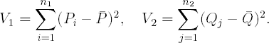
Fligner and Policello (Fligner and Policello, 1981) suggested the following test to compare two location parameters from distributions with differing amounts of variation. The statistic is based upon a quantity called a placement. A placement is the number of values in one sample strictly less than a given value of a secondsample. Consider samples X1,...,Xn1 and Y1,...,Yn2. For a value Xi, i = 1,..., n1, its corresponding placement, Pi, is the number of values from Y1,..., Yn2 less than Xi. Similarly, for a value Yj, j = 1,..., n2, its placement, Qj, is the number of values from the first sample less than Yj. The next steps involve calculating quantities similar to those required for a standard Student's two-sample t-test. To perform the hypothesis test
- H0 : δ = 0 when ϕ1 ≠ ϕ2 versus HA : δ > 0 when ϕ1 ≠ ϕ2,
we need to compute the average placements, ![]() and
and ![]() , as well as the variances:
, as well as the variances:
The Fligner-Policello test statistic is of the form:
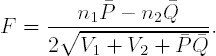
We reject H0 in favor of HA at level α if F ≥ cα, where cα is the cutoff from the null distribution of the Fligner-Policello statistic. By the Central Limit Theorem, F ~ N(0,1), cα may be conveniently replaced with the quantile from a standard normal distribution, zα, when n1 and n2 are large. This gives us the large-sample versions of the lower and two-tailed tests, respectively:
Reject H0 : δ = 0 (when ϕ1 ≠ ϕ2) in favor of HA : δ < 0 (when ϕ1 ≠ ϕ2) if F ≤ −zα.
Reject H0 : δ = 0 (when ϕ1 ≠ ϕ2) in favor of HA : δ ≠ 0 (when ϕ1 ≠ ϕ2) if|F| ≥ zα/2.
If ties exist in the data, one needs to adjust the Fligner-Policello statistic defined above. The adjustment occurs at the level of the placements. When calculating one set of the placements, for example, to compute Pi, we count the number of the Y's less than Xi and add half of the values equal to Xi. The same is true for the other set of placements. The balance of the method remains unchanged.
6.2.3.3. %FPSTATISTIC Macro for Performing the Comparison of Two Location Parameters in the Absence of Unequal Scale
The %FPSTATISTIC macro, available on the book's companion Web site, performs the large sample version of the Fligner-Policello test. To invoke the macro, the user needs to specify three parameters:
DATASET is the name of the data set.
VAR is the name of the response variable.
GROUPVAR is the name of the grouping (classification) variable for the macro. This variable must have only two levels.
The macro begins by determining the sample size for each level of the grouping variable. After the macro determines the two group sample sizes, it begins to calculate the placements for each group including an adjustment for ties. The algorithm involves a loop that iteratively compares values and assigns an indicator variable with the values 1 (greater than response in other group), 0.5 (tied or equal values) or 0 (for less than response in other group). These indicators are added to form the placements for the first group with n1 observations. The same procedure is followed for the n2 placements of the second group.
The final portion of the macro uses MEANS procedure to calculate the sum of the placements, mean placements, and corrected sums of squares for the placements for each level of the grouping variable. The PROBNORM function is then used to determine the p-values. The macro outputs three versions of the large sample Fligner-Policello test, two-sided, upper and lower (the results are saved in the FPSTATISTIC data set).
Program 6.6 calls the %FPSTATISTIC macro to perform a comparison of the blood bacterial count data in the placebo and treated groups. Note that the location parameters for the two levels of the classification variable are compared in reverse alphanumeric sort order. Thus, for the BBC data set, the macro will test whether the location parameter in the treated group is greater than the location parameter in the placebo group. In the antibacterial trial example, we are interested in knowing if the treatment lowered the blood bacterial count. Thus we need to focus on the one-sided, lower-tailed test.
Example 6-6. Fligner-Policello test in the antibacterial trial example
%fpstatistic(dataset=bbc,var=bbc,groupvar=group);
proc print data=fpstatistic noobs label split="*";
    format uhat 6.3 p2sided up1sided low1sided 5.3;
    var n1 n2 uhat p2sided up1sided low1sided;
run; |
Example. Output from Program 6.6
Sample     Sample
      size       size        FP        Two-sided    Upper-tailed    Lower-tailed
    group 1    group 2    statistic     p-value       p-value         p-value

109 184 −1.615 0.106 0.947 0.053 |
Output 6.6 shows that the one-sided lower-tailed p-value is not significant at a 0.05 level (p = 0.053). Thus the Fligner-Policello test fails to reject the null. We conclude that there is not enough evidence to declare the blood bacterial counts to be statistically significantly different between the two treatment groups. The results of this analysis are much more in agreement with the summary statistics presented earlier in Table 6.2.
6.2.3.4. Role of Data Transformations
It is very common for data analysts to employ basic transformations on data so that the transformed data will have desirable properties. Two common means of transforming data are the use of logarithms and rank-transformations. Logarithmic transformations are not always useful, as zeros or negative values may exist in data sets. Moreover, applying a logarithmic transformation to data, followed by performing a two-sample Student's t-test, does not always test the desired hypothesis comparing the locations of two samples' distributions (see Zhou et al., 1997, for a discussion of this practice).
Some folklore has evolved amongst practitioners of statistical methods in the field with respect to the rank-transformations. A common misconception is that the rank-transform eliminates the need to adjust for unequal dispersion, i.e., the rank-transformation corrects for the problem of unequal variation. As illustrated previously, the results of performing a rank-transformation and a large-sample approximate Wilcoxon Rank Sum test may produce a counter-intuitive inference. The author would recommend the application of the Fligner-Policello method in an analysis of two independent samples where the distributions are believed to differ in scale.
Although, on the surface, the analysis of the two independent samples seems trivial, the setting still requires the care necessary for any data analysis. The features of the data must be understood and matched appropriately to the assumptions of the statistical method(s) employed. This is a theme that will be reiterated more times throughout this chapter.
Now that we have examined a few aspects of the two independent samples case, it is time to advance to the setting of k independent samples. The next section will address several nonparametric approaches to analyzing data in this common experimental setting, largely emphasizing examples from drug discovery research.
6.2.4. Summary
The two-sample problem is not unlike other problems in statistical inference: careful examination of the assumptions is required to execute an appropriate analysis. Nonparametric statistics methods afford techniques for handling the comparison of two distributions' locations in both the case of similar dispersion (Wilcoxon Rank Sum test) and differing dispersion (Fligner-Policello test). In the case of the former, the corresponding analysis may be carried out with PROC NPAR1WAY. In the latter case, the analysis may be executed with a SAS macro created by the author (%FPSTATISTIC macro).