7.4. Regression Models with Unknown Parameters in the Variance Function

In various pharmaceutical applications it is often assumed that the variance of the error term, σ², depends not only on the control variable x, but also on the unknown parameter θ, i.e., σ_i² = S(x_i,θ).

Consider, for instance, the four-parameter logistic model introduced in Section 7.2. The variance of the response variable, Y, may depend on its mean, as in the following power model (Finney, 1976; Karpinski, 1990; Hedayat et al, 1997):

In cell-based assay studies, the response variable is a cell count and is often assumed to follow a Poisson distribution. Under this assumption, one can consider a power variance model with δ = 1.

Another possible generalization of the nonlinear regression models considered in Section 7.2 is a regression model with multiple correlated responses. Multiple correlated responses are encountered in clinical trials with several endpoints or several objectives, e.g., simultaneous investigation of efficacy and toxicity in dose response studies (Heise and Myers, 1996; Fan and Chaloner, 2001).

7.4.1. General Model

Let the observed response Y be a normally distributed k-dimensional vector with

where η(x,θ) = (η₁(x,θ),...,η_k(x,θ))^T is a vector of pre-defined functions and s(x,θ) is a k × k positive definite matrix. It can be shown that the Fisher information matrix of a single observation, μ(x,θ), is the sum of two terms; see Magnus and Neudecker, 1988, Chapter 6, or Muirhead, 1982, Chapter 1:

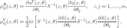
where m is the number of unknown parameters. In the univariate case (k = 1), μ(x,θ) permits the following factorization:

where

f(x,θ) is the vector of partial derivatives of η(x,θ) as in (7.10) and h(x,θ) is the vector of partial derivatives of S(x,θ) with respect to θ, i.e.,

It is important to note that, since the information matrix μ(x,θ) consists of two terms, its rank may be greater than 1 even in the univariate case. This may lead to the situation when the number of support points in the optimal design is less than the number of unknown parameters, i.e., less than m (see Downing, Fedorov and Leonov (2001) or Fan and Chaloner (2001) for examples). This cannot happen in regression models with a single response variable and a known variance since in this case the information matrix of the design would become singular.

7.4.1.1. Sensitivity Functions

Using classic optimal design techniques, it can be shown that the equivalence theorem (7.6), (7.7) remains valid for multivariate models in which the covariance matrix depends on unknown parameters (Atkinson and Cook, 1995; Fedorov, Gagnon and Leonov, 2002). In the univariate case, sensitivity functions for the D- and A-optimality criteria can be presented as the sum of two terms and can be factorized too. For example, the sensitivity function for the D-optimality criterion can be written as

7.4.2. Example 4: A Four-Parameter Logistic Model with a Power Variance Model

This example is concerned with the computation of the D-optimal design in a four-parameter logistic model that extends the logistic model considered in Example 3 (see Section 7.3). Assume that Y is a normally distributed response variable with

where δ₁ and δ₂ are positive parameters.

Parameters θ₁ − θ₄ are selected as in Example 3, i.e., θ = (15.03, 1.31, 530, 1587)^T and δ₁ = 0.5, δ₂ = 1. The combined vector of model parameters is (15.03, 1.31, 530, 1587, 0.5, 1)^T.

7.4.2.1. Computation of the D-Optimal Design

Program 7.4 computes the D-optimal design for the four-parameter logistic model specified above. This program is conceptually similar to Program 7.3, We need only to make the following changes:

• Add the two variance parameters to the PARAMETER variable.

• Change the method of calculating the derivatives since the analytic form of the derivatives is rather complicated. The %deriv macro computes gR(x,θ) numerically using the NLPFDD function. Since the information matrix and sensitivity function also depend on gV(x,θ), we introduce a new macro (%derivs) that calculates this function gV(x,θ) (it is also derived using a numerical approximation).

• Since the information matrix is now the sum of two terms, the %infod macro needs to be modified as well.

• As in Program 7.3, the value of the merging constant (CMERGE) is increased to improve the stability of the iterative procedure in this complex optimal design problem.

The complete version of Program 7.4 is provided on the book's companion web site.

Example 7-4. D-optimal design for the four-parameter logistic model with a continuous response and unknown parameters in the variance function (Design and algorithm parameters)

* Design parameters;
%let points=do(-0.024,6.215,6.239/7);
%let weights=repeat(0.125,1,8);
%let grid=do(-0.024,6.215,6.239/400);
%let parameter={15.03 1.31 530 1587 0.5 1};
* Number of parameters;
%let paran=6;

* Algorithm parameters;
%let convc=1e-9;
%let maximit=1000;
%let const1=1;
%let const2=1.2;
%let cmerge=7.5;
%OptimalDesign1;

Example. Output from Program 7.4

Initial design

                                  Weight         X

                                   0.125    −0.024
                                   0.125     0.867
                                   0.125     1.759
                                   0.125     2.650
                                   0.125     3.541
                                   0.125     4.432
                                   0.125     5.324
                                   0.125     6.215

                                   Optimal design

                                  Weight         X

                                   0.294    −0.024
                                   0.213     1.972
                                   0.236     3.563
                                   0.257     6.215

Output 7.4 lists the initial and optimal designs. Other parameters of the two designs, e.g., the variance-covariance matrices and their determinants, can be obtained by printing out the DINITIAL, DOPTIMAL and DDET data sets. It was emphasized above that, in models with unknown parameters in the variance function, the number of support points in optimal designs can be less than the number of model parameters. Indeed, Output 7.4 shows that, although there are two more unknown parameters in this model compared to the model with a constant variance (Example 3 of Section 7.3), the D-optimal design is still a four-point design. The weights are no longer equal to 1/4, and are equal to (0.294,0.213,0.236,0.257) for the four design points (−0.024,1.972,3.563,6.215) on the log-scale.

Figure 7.6 provides a visual comparison of the initial and optimal designs (left panel) and also plots the sensitivity functions associated with the two designs (right panel).