7.8. Pharmacokinetic Models with Multiple Measurements per Patient

In this section we discuss a clinical pharmacokinetic (PK) study where multiple blood samples are taken for each enrolled patient. This setup leads to nonlinear mixed effects regression models with multiple responses.

7.8.1. Two-Compartment Pharmacokinetic Model

Consider a clinical trial in which the drug was administered as a bolus input D₀ at the beginning of the study (at time x = 0) and then bolus inputs D_i were administered at 12 or 24 hour intervals until 72 hours after the first dose. To describe the concentration of drug at time x, a two-compartment model was used with standard parameterization (volume of distribution V, transfer rate constants K₁₂, K₂₁ and K₁₀), see Figure 7.14.

Figure 7-13. Left panel: Initial (open circles) and optimal (closed circles) designs. Right panel: Sensitivity functions for the initial (dashed curve) and optimal (solid curve) designs.

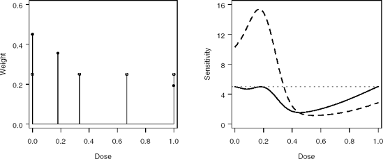
Figure 7-14. Diagram of the two-compartment model

Measurements of drug concentration y_ij were taken from the central compartment (compartment 1 in Fig. 7.14) at times x_j for each patient,

g₁(x_j) = g₁(x_j,γ_i) is the amount of the drug in the central compartment at time x_j for patient i, γ_i = (V_i,K_12,i,K_21,i,K_10,i) are individual PK parameters of patient i and z_ij are measurement errors. The g₁ function and population model are discussed in more detail below.

In the trial under consideration k = 16 samples were taken from each patient at times x_j ∈ χ,

Obviously, each extra sample provides additional information and increases the precision of parameter estimates. However, the number of samples that may be drawn from each patient is restricted because of blood volume limitations and other logistical and ethical reasons. Moreover, the analysis of each sample is associated with monetary costs. Therefore, it is reasonable to take the cost of drawing samples into account. If X = (x₁,..., x_k) is a collection of sampling times for a particular patient, we can consider the cost of the sampling sequence X (denoted by c(X)).

In this section we will consider the following questions:

By an optimal sampling scheme we mean a sequence which allows us to obtain the best precision of parameter estimates in terms of their variance-covariance matrix and the selected optimality criterion. First, we need to define the regression model with multiple responses, see (7.11). In this and next sections, X will denote a k-dimensional vector of sampling times and Y will be a k-dimensional vector of measurements at times X.

7.8.2. Regression Model

A two-compartment model described by the following system of linear differential equations was used to model the data:

for x ∈ [t_i,t_i+1) with initial conditions

where q₁(x) and q₂(x) are amounts of the drug at time x in the central and peripheral compartments, respectively; t_i is a time of i-th bolus input, t₀ = 0; D_i is the amount of the drug administered at t_i.

The solution of the system (7.19) is a sum of exponential functions which depend on parameters (Gibaldi and Perrier, 1982, Appendix B):

In population modeling it is often assumed that the γ_i parameters for patient i are independently sampled from the normal population with

where the m_γ-dimensional vector γ⁰ and (m_γ × m_γ) matrix Λ are usually referred to as the "population", or "global", parameters; see Gagnon and Leonov (2005) for a discussion on other population distributions.

To fit the model, it was assumed that the variance of the error term z_ij in (7.18) depends on the model parameters through the mean response,

where ε_1,ij and ε_2,ij are independent, identically distributed random variables with zero mean and variance σ₁² and σ₂², respectively.

Let θ = (γ⁰,Λ, σ₁²,σ₂²) denote a combined vector of model parameters and k_i denote the number of samples taken for patient i. Let

be sampling times and measured concentrations, respectively, for patient i. Further, η(x_ji,γ_i) = q₁(x_ji,γ_i)/V_i, η(x_ji,θ) = q1(x_ji,γ⁰)/V and

where j = 1,2,...,k_i.

If F is a (k_i × m_γ) matrix of partial derivatives of function η(X_i,θ) with respect to parameters γ₀,

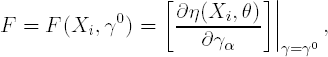
then, using the first order approximation together with (7.20) and (7.21), one obtains the following approximation of the variance-covariance matrix S(X_i,θ) for Y_i,

where Diag(A) denotes a diagonal matrix with elements a_ii on the diagonal; see also Fedorov, Gagnon and Leonov (2002; Section 4). If the γ parameters are assumed to be log-normally distributed, then Λ on the right-hand side of (7.22) has to be replaced with

for details, see Gagnon and Leonov (2005). Therefore, for any sequence X_i, the response vector η(X_i,θ) and variance-covariance matrix S(X_i,θ) are defined, and we can use general formula (7.12) to calculate the information matrix μ(X_i,θ).

7.8.3. Example 9. Pharmacokinetic Model without Cost Constraints

Consider a problem of selecting an optimal sampling scheme with a single bolus input at time x = 0. SAS code for generating optimal designs for the general case of multiple bolus inputs is available (Gagnon and Leonov, 2005), but the complexity of this code is beyond the scope of the chapter.

To fit the data, the K₁₂ and K₂₁ parameters were treated as constants (K₁₂ = 0.400, K₂₁ = 0.345), i.e., they were not accounted for while calculating the information matrix μ(x,θ). Therefore, the combined vector of unknown parameters θ was defined as

where

CL is the plasma clearance and K₁₀ = CL/V. The total number of unknown parameters is m = 7.

To construct locally optimal designs, we obtained the parameter estimates using the NONMEM software (Beal and Sheiner, 1992) based on 16 samples (from the design region χ) for each of 27 subjects. The resulting estimate is given by

Drug concentrations were expressed in μg/L, elimination rate constant K₁₀ in L/h and volume V in L.

The PK modeling problem considered in this section greatly increases the complexity of the SAS implementation of D-optimal designs. Program 7.9 relies on a series of SAS macros and SAS/IML modules to solve the optimal selection problem formulated earlier in this section. Referring back to Section 7.1.7, Components 1, 2 and 3 of the general optimal design algorithm require extensive changes. These changes are summarized below.

• In order to generate the grid, the set of sampling times χ is defined in the CAND data set and the number of time points r in the final design is specified in the KS data set (in this case, we are looking for 8-point designs). Note that r ranges between 1 and k, where k is the total number of sampling times (k = 16 in this case). Any number of sets of size r can be applied to the optimization algorithm; however, for designs with the standard information matrix normalization, the design with the largest r will be D-optimal. This will not (necessarily) be true for cost normalized designs (see Section 7.9).

• The problem of selecting candidate points is a C(k,r) problem, where C(k,r) is a binomial coefficient, C(k,r) = k!/[r!(k - r)!]. Sets of size r candidate points can become very large. For example, for k = 16 and r = 8, the number of possible 8-point sampling schemes is C(16,8) = 12,870 which means that 12,870 information matrices need to be obtained. Note that in this example m = 7 and thus each information matrix is a 7 × 7 matrix. In order to store the information matrices for all possible 8-point designs, SAS needs to store 12,870 × 7 = 90,090 rows (and 7 columns) of data. Hence the data storage requirements for large designs can become formidable. Once the CAND and KS data sets are specified, Program 7.9 will generate the set of possible candidate points using the SAS/IML module TS. Also, the initial design is specified in the SAMPLE data set (note that all points in the initial design must be elements of the design region χ and must be of length r, as specified in the KS dataset).

• The set of parameters has been defined as θ = (γ₁⁰,γ₂⁰,λ₁₁,λ₂₂,λ₁₂,σ₁²,σ₂²).^T Since we are dealing with a mixed effects model, the γ and λ parameters in the vector θ must be identified. This is accomplished by ordering the parameters in a specific way. In general, the parameters in θ must be entered as follows: vector γ, vector λ, and residual variance(s). The number of components in γ is defined by the NF macro variable. The ordering of the random effects (the λ's) is also highly important. Parameters along the main diagonal of Λ should be entered first: λ₁₁,λ₂₂. The off-diagonal element (λ₁₂) should be entered next. The Λ matrix is set up using the SAS/IML module LSETUP. In the general case, when Λ is a b × b matrix, the components of Λ need to be ordered as follows: diagonal elements, λ₁₁,λ₂₂,...,λ_bb, followed by off-diagonal elements λ₁₂,λ₁₃,...,λ_1b, λ₂₃,λ₂₄,λ_2b,..., etc.

• The PK function, η(x,θ), derived from (7.19), is specified using the SAS/IML module FPARA. The ordering of the γ's in the vector of parameters must match the ordering in the FPARA module. As shown in Program 7.9, CL (plasma clearance) should be entered into θ first, and V (volume of distribution) should be entered second. In the current version, the equations in (7.19) must be solved, and the solution must be entered in the FPARA module.

• A computationally difficult issue is the calculation of derivatives for (7.12). Note that first- and second-order partial derivatives are required; see equations (7.12), (7.22). In the previous examples derivatives were obtained by either entering the analytical form or by using the NLPFDD function in SAS/IML. Here, we find it more practical to calculate the derivatives numerically using the following approximation

  
  

  where the value of h is a macro variable and is entered by the user (h = 0.001 in this example). The information matrix from (7.12) is computed via the SAS/IML module MOLD, which calls six other modules (HIGHERD, HIGHERM, FPLUS, FMINUS, FTHETA and JACOB2).

The complete SAS code for this example is provided on the book's companion Web site.

Example 7-9. D-optimal design for the pharmacokinetic model (Design and algorithm parameters)

* Design parameters;
%let h=0.001;  * Delta for finite difference derivative approximation;
%let paran=7;  * Number of parameters in the model;
%let nf=2;     * Number of fixed effect parameters;
%let cost=1;   * Cost function (1, no cost function,
                                2, user-specified function);
* Algorithm parameters;
%let convc=1e-9;
%let maximit=1000;
%let const1=2;
%let const2=1;
%let cmerge=5;
* PK parameters;
data para;
    input CL V vCL vV covCLV m s;
    datalines;
    0.211 5.50 0.0365 0.0949 0.0443 0.0213 8060
    ;
* All candidate points;
data cand;
    input x @@;
    datalines;
    0.083 0.25 0.5 0.75 1 2 3 4 5 6 12 24 36 48 72 144
    ;
* Number of time points in the final design;
data ks;
    input r @@;
    datalines;
    8
    ;
* Initial design;
data sample;
    input x1 x2 x3 x4 x5 x6 x7 x8 w @@;
    datalines;
    0.083 0.5 1 4 12 24 72 144 1.0
    ;
    run;

Example. Output from Program 7.9

Determinant of the covariance matrix D (initial design)

                                         IDED

                                      0.0000136

                 Determinant of the covariance matrix D (final design)

                                         DETD

                                      8.4959E-6

                                  Optimal design

             COL1    COL2    COL3    COL4    COL5    COL6    COL7    COL8

            0.083    0.25     0.5    0.75     36      48      72      144

Output 7.9 lists the optimal sampling times included in a D-optimal 8-point design (5 min, 15 min, 30 min, 45 min, 36 h, 48 h, 72 h and 144 h). The optimal design differs from the initial design in that it puts more weight on earlier time points, e.g., the optimal design includes the 15-min and 45-min which were not in the initial design. Note also that an application of the D-optimal algorithm reduced the determinant of the optimal variance-covariance matrix to 8.49 × 10⁻⁶ (from 1.36 × 10⁻⁵).