
14.7. Selection of an Optimal Dose
One of the most crucial decisions in the development of a new drug is which dose to use. The situation varies between different indications. Sometimes the dose can be titrated for each patient, sometimes the dose is individualised based on gender, body weight, genetic constitution and other factors. Often one looks for a one-dose-fits-all. The optimal dose is a compromise between beneficial effects and undesired side effects. In general, both effects and, especially, side effects, may be multi-dimensional. As a further complication, which side effects are important may not be clear until after the Phase III programme or even after marketing of the drug. We choose to treat only the simple situation with a one-dimensional effect variable and a one-dimensional, well specified type of adverse event. A practical example of finding the optimal dose, based on decision analysis and modeling of efficacy and safety, is provided by Graham et al (2002).
Effects and side-effects are typically measured on different scales and defining the optimal dose requires that they are weighted together in some way. It is, however, not obvious how to weigh a decrease in blood pressure against a risk of severe coughing, or how to weigh a decrease in body weight against problems with loose stools. Although such weighting has to be subjective, there is no rational way to avoid it. Given dose-response information for effects and adverse events, to choose a dose more or less implies at least an implicit statement about the relative importance of the two dimensions.
On some occasions, it may occur that effects and side effects can be measured directly on the same scale. One example is when both the effect and the side effect are measured in terms of lives and dying. Even though effects and side effects appear to be measured on the same scale, it is not obvious that they should be weighted equally. Different causes of death may give different opportunities for the patient to prepare for death. Even if the outcomes are identical in almost everything, it may subjectively be harder to accept negative events due to the treatment than similar negative events due to the natural propagation of the disease. Furthermore, there may be a legal difference: it is easier to blame the doctor for a treatment's adverse effects than for the negative effects of the untreated disease. Thus, a weighting of adverse effects relative beneficial effects is generally needed.
Suppose that the effect is a continuous variable and the adverse effect is dichotomous. Let E(D) be the expected effect and p(D) the probability that a patient experiences an AE, as functions of the dose D. One reasonable utility function is the simple weighted combination
Since it is often hard to choose a value of the weight k, it is useful to investigate the robustness of the conclusions over a range of values of k.
A common model for the effect is the so called Emax model
The parameters E0, Emax and ED50 have natural interpretations as placebo response, the maximal possible placebo-adjusted effect and the dose for which the adjusted effect is 50% of Emax, respectively. The Hill coefficient γ is related to the steepness of the dose-response curve around ED50.
Knowledge of the effect curve alone does not imply what the optimal dose is; safety information is also needed. Assume a logistic model for the probability of AE as a function of the logarithm of the dose,

14.7.1. Models without Uncertainty
First, assume all parameters to be fixed, Here is an example:
Assume also that the weight k = 1000, meaning that 0.1% AEs is equalised to one unit of effect. Program 14.12 examines the relationship between the dose of an experimental drug D and the expected effect E(D), adverse event probability p(D) and utility U(D).
Example 14-12. Plot of the dose-effect, dose-Prob(AE) and dose-utility functions
/* Define model parameters and macros */
%let k=1000;
%let emax=300;
%let ed50=0.3;
%let gamma=1.0;
%let e0=0.0;
%let alpha=-1.5;
%let beta=2.0;
%macro effmodel(dose,emax,ed50,gamma,e0);
    %global effout;
    %let effout=&e0+&emax*&dose**&gamma/(&dose**&gamma+&ed50**&gamma);
%mend effmodel;
%macro AEmodel(logdose,alpha,beta);
    %global AEout;
    %let AEout=exp(&alpha+&beta*&logdose)/(1+exp(&alpha+&beta*&logdose));
%mend AEmodel;
/* Create data set for plotting */
data window;
    do logd=log(0.01) to log(10.0) by log(10.0/0.01)/100;
        dose=exp(logd);
        %effmodel(dose=dose,emax=&emax,ed50=&ed50,gamma=&gamma,e0=&e0);
        effect=&effout;
        %AEmodel(logdose=logd,alpha=&alpha,beta=&beta);
        AEprob=&AEout;
        AEloss=&k*AEprob;
        utility=effect-AEloss;
        output;
    end;
axis1 minor=none label=(angle=90 "Utility") order=(-300 to 300 by 100);
axis2 minor=none label=("Dose") logbase=10 logstyle=expand;
symbol1 i=join width=3 line=1 color=black;
symbol2 i=join width=3 line=20 color=black;
symbol3 i=join width=3 line=34 color=black;
proc gplot data=window;
    plot (effect AEloss utility)*dose/haxis=axis2 vaxis=axis1
    overlay frame vref=0 lvref=34;
    run;
quit; |
Figure 14.11 displays the dose-effect, dose-Prob(AE) and dose-utility functions. It is clear that the first two functions, E(D) and p(D), are monotone functions of the dose. By contrast, the dose-utility function is increasing on [0,D*] and decreasing on [D*,10], where D* is the dose that maximizes the utility function. The optimal dose, D*, is easy to find using PROC NLP (see Program 14.13).
Figure 14-11. Plot of the dose-effect (solid curve), dose-Prob(AE) (dashed curve) and dose-utility (dotted curve) functions

Example 14-13. Computation of the optimal dose
proc nlp outest=result noprint;
    max utility;
    decvar dose;
    %effmodel(dose=dose,emax=&emax,ed50=&ed50,gamma=&gamma,e0=&e0);
    effect=&effout;
    %AEmodel(logdose=log(dose),alpha=&alpha,beta=&beta);
    AEprob=&AEout;
    utility=effect-&k*AEprob;
data result;
set result;
format optdose effect utility 6.2 AEprob 5.3;
where _type_="PARMS";
optdose=dose;
%effmodel(dose=optdose,emax=&emax,ed50=&ed50,gamma=&gamma,e0=&e0);
effect=&effout;
%AEmodel(logdose=log(optdose),alpha=&alpha,beta=&beta);
AEprob=&AEout;
utility=effect-&k*AEprob;
label optdose="Optimal dose"
effect="Effect"
AEprob="Probability of an AE"
utility="Utility";
keep optdose effect AEprob utility;
proc print data=result noobs label;
run; |
Example. Output from Program 14.13
Optimal                         Probability
                            dose      Effect    Utility     of an AE

0.42 175.02 137.13 0.038 |
Output 14.13 lists the optimal dose, expected response, utility and, finally, probability of observing an AE at this dose. The optimal dose is D* = 0.42, and the associated net utility is given by
14.7.2. Choosing the Optimal Dose Based On Limited Data
In reality, the efficacy and safety models considered above are uncertain and have to be estimated from the information at hand. We will assume that a relatively small dose-finding trial (124 patients) has been run to study the efficacy and safety of five doses of an experimental drug. The data collected in the study (DOSE, EFF and AE variables) are contained in the STUDY data set available on the book's companion web site. The AE variable is 1 for patients who have experienced the AE, and 0 otherwise. The EFF variable is the observed effect. Table 14.1 displays the summary of the efficacy and safety data in the STUDY data set.
| Dose | Number of patients | Number of AEs | Efficacy variable | |
|---|---|---|---|---|
| Mean | SD | |||
| 0.03 | 26 | 0 | −13.7 | 291.8 |
| 0.1 | 23 | 0 | 135.6 | 269.3 |
| 0.3 | 25 | 1 | 132.6 | 267.0 |
| 1 | 26 | 5 | 293.0 | 328.3 |
| 3 | 24 | 10 | 328.4 | 339.1 |
In addition to this limited information on the new drug's effect, there is a lot of literature data for other drugs from the same class. Based on this, we think that we can estimate the E0, Emax and γ parameters of the Emax model, introduced earlier in this section, sufficiently well. (it is assumed that the parameters are shared by all drugs in the class). Thus, we will take E0 = 0, Emax = 300 and γ = 1.0 as fixed. Only the potency, described by ED50, of our new drug remains uncertain. The computations are simplified as only one of the four parameters in the Emax model must be estimated based on the small in-house trial.
Before estimating the unknown parameters, ED50, α and β, it is good to consider how reliable the efficacy and safety models are. Even if the models fit the data well, we should not be over-confident. For example, it is often possible to fit logit, probit and complementary log-log models to the same data set. Still, these models have a large relative difference in the predicted probability of AE at very low doses. In our example, as in many practical situations, there is not enough data to discriminate between different reasonable types of models. A model-independent analysis is therefore a good start.
Program 14.14 calculates estimates (EFF_MEAN, UTIL_EST, P_EST) and their standard errors (EFF_SE, UTIL_SE, P_SE) for mean effect, mean utility, and probability of an AE, respectively, in each of the five dose groups. Note that, depending on the nature of the effect and AE variables, it is plausible that they are positively or negatively correlated. For the sake of simplicity, however, we assume independence throughout this section. This assumption may alter the estimated standard error for the utility but is unlikely to have a major impact on the estimated mean utility.
Example 14-14. Model-free estimates and SEs of E(D), p(D) and U(D)
%let k=1000;              /* Weighting coefficient */
proc means data=study.study;
    class dose;
    var eff;
    output out=summary_eff(where=(_type_=1)) n=n mean=mean std=std;
proc freq data=study.study;
    table dose*ae/out=summary_ae(where=(ae=1));
data summary;
    merge summary_eff summary_ae;
    by dose;
    if count=. then count=0;
    n_ae=count;
eff_mean=mean;
eff_sd=std;
keep dose n n_ae eff_mean eff_sd;
data obs_util;
set summary;
format eff_mean eff_se util_est util_se 5.1 p_est p_se 5.3;
eff_se=eff_sd/sqrt(n);
p_est=n_ae/n;
p_se=sqrt(p_est*(1-p_est)/n);
util_est=eff_mean-&k*p_est;
util_se=sqrt(eff_se**2+(&k*p_se)**2);
label dose="Dose"
eff_mean="Effect"
eff_se="Effect (SE)"
p_est="Probability of an AE"
p_se="Probability of an AE (SE)"
util_est="Utility"
util_se="Utility (SE)";
keep dose eff_mean eff_se p_est p_se util_est util_se;
proc print data=obs_util noobs label;
run; |
Example. Output from Program 14.14
Probability
                            Effect               Utility    Probability     of an AE
          Dose    Effect     (SE)     Utility     (SE)       of an AE         (SE)

          0.03    −13.7      57.2      −13.7       57.2        0.000          0.000
          0.10    135.6      56.2      135.6       56.2        0.000          0.000
          0.30    132.6      53.4       92.6       66.2        0.040          0.039
          1.00    293.0      64.4      100.7      100.6        0.192          0.077
3.00 328.4 69.2 −88.3 122.1 0.417 0.101 |
Output 14.14 lists the three estimated quantities (mean effect, mean utility and probability of an AE) along with the associated standard errors. The highest observed utility is for Dose 0.1. For this dose, the utility is significantly better than placebo (as the z-score is 135.6/56.2 ≈ 2.42). Considering the large standard errors, however, it is hard to distinguish between doses in a large range. The only immediate conclusion is that the optimal dose should be higher than 0.03 and probably lower than 3.
After using a model-free approach, we proceed to fit the Emax model to the efficacy data and logistic model to the safety data. Program 14.15 uses the NLIN and LOGISTIC, respectively, to calculate parameter estimates in the two models. The parameter estimates are assigned to macro variables for use later.
Example 14-15. Estimating parameters and posterior distribution
data studylog;
    set study;
    logdose=log(dose);
%let e0=0;
%let emax=300;
%let gamma=1.0;
proc nlin data=study outest=estED50;
ods select ParameterEstimates;
parms log_ed50=-1;
model eff=&e0+&emax*dose**&gamma/(dose**&gamma+exp(log_ed50)**&gamma);
output out=Statistics Residual=r parms=log_ed50;
data estED50;
set estED50;
if _type_="FINAL" then
call symput('log_est',put(log_ed50, best12.));
if _type_="COVB" then
call symput('log_var',put(log_ed50, best12.));
run;
proc logistic data=studylog outest=est1 covout descending;
ods select ParameterEstimates CovB;
model ae=logdose/covb;
data est1;
set est1;
if _type_='PARMS' then do;
call symput('alpha_mean',put(intercept, best12.));
call symput('beta_mean',put(logdose, best12.));
end;
else if _name_='Intercept' then do;
call symput('alpha_var',put(intercept, best12.));
call symput('ab_cov',put(logdose, best12.));
end;
else if _name_='logdose' then call symput('beta_var',put(logdose, best12.));
run; |
Example. Output from Program 14.15
The NLIN Procedure

                                        Approx      Approximate 95% Confidence
          Parameter      Estimate    Std Error                Limits

          log_ed50        −1.5794       0.5338     −2.6360     −0.5228

                             The LOGISTIC Procedure

                   Analysis of Maximum Likelihood Estimates

                                     Standard          Wald
      Parameter    DF    Estimate       Error    Chi-Square    Pr > ChiSq

      Intercept     1     −1.6566      0.3435       23.2639        <.0001
      logdose       1      1.2937      0.3487       13.7647        0.0002

                          Estimated Covariance Matrix

                     Variable       Intercept       logdose

                     Intercept       0.117968      −0.05377
logdose −0.05377 0.1216 |
Output 14.15 lists the estimated model parameters. Note that a direct estimation of ED50 (not shown) will result in a 95% confidence interval which contains negative values. Such values are not plausible. As the uncertainty in the parameter estimates will be important later, we prefer to estimate log(ED50) rather than ED50. The estimate and sample standard error of log(ED50) are −1.5794 and 0.5338, respectively.
The estimates of α and β in the logistic model for the probability of observing an AE are ![]() = −1.6566 and
= −1.6566 and ![]() = 1.2937, respectively. The covariance matrix is governed by
= 1.2937, respectively. The covariance matrix is governed by
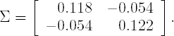
One obvious way to consider the parameter uncertainty is to apply a Bayesian viewpoint and consider the posterior distributions for the parameters. The posterior distribution is proportional to the prior multiplied by the likelihood. PROC LOGISTIC and PROC NLIN are likelihood-based procedures and the output from them can be used to get at least rough approximations of the likelihood functions. Assuming that the priors are relatively flat, we may take the two-dimensional normal distribution with mean
and covariance matrix Σ as the approximate posterior for

Similarly, the estimate of log(ED50) and its standard error may, to a reasonable approximation, serve as the mean and standard deviation in a normal prior for log(ED50).
Program 14.16 uses the previously calculated macro variables to simulate utility curves based on the posteriors for the parameters. Figure 14.12 displays a number of simulated curves together with the simulated expected utility curve.
Example 14-16. Estimating parameters and posterior distribution
%let nsim=1000;     /* Number of simulated curves */
%let ndisplay=10;   /* Number of displayed individual curves */
%let doseint=100;   /* Dissolution of dose scale */
%macro out_sim;
    %do __cnt=1 %to &ndisplay.;
        simu&__cnt.=t(util_sim[&__cnt.,]);
    %end;
    create simdata var{dose logdose Eutility
        %do __cnt=1 %to &ndisplay.; simu&__cnt. %str( ) %end;};
    append;
%mend out_sim;
%macro ind_plot;
    %do __cnt=1 %to &ndisplay.;
        simu&__cnt.*dose
    %end;
%mend ind_plot;
/* Simulations */
proc iml;
    seed=257656897;
    z=normal(repeat(seed,&nsim,3));
    alpha_sd=sqrt(&alpha_var);
    beta_sd=sqrt(&beta_var);
    ab_corr=&ab_cov/sqrt(&alpha_var*&beta_var);
    alpha_sim=&alpha_mean+alpha_sd*z[,1];
    beta_sim=&beta_mean+beta_sd*(ab_corr*z[,1]+sqrt(1-ab_corr**2)*z[,2]);
    logED50_sd=sqrt(&log_var);
    logED50_sim=&log_est+logED50_sd*z[,3];
    ED50_sim=exp(logED50_sim);
logdose=t(do(log(0.01),log(10),log(10/0.01)/&doseint));
logdosematrix=j(&nsim,1)*t(logdose);
dose=exp(logdose);
dosematrix=exp(logdosematrix);
onevector=j(1,nrow(logdose));
alpha_sim_matrix=alpha_sim*onevector;
beta_sim_matrix=beta_sim*onevector;
ED50_sim_matrix=ED50_sim*onevector;
logit=exp(alpha_sim_matrix+beta_sim_matrix#logdosematrix);
prob_sim=logit/(1+logit);
Eprob=t(j(1,&nsim)*prob_sim/&nsim);
effect_sim=&e0+&emax*dosematrix##&gamma/
(dosematrix##&gamma+ED50_sim_matrix##&gamma);
Eeffect=t(j(1,&nsim)*effect_sim/&nsim);
util_sim=effect_sim-&k*prob_sim;
Eutility=t(j(1,&nsim)*util_sim/&nsim);
/* Create data set containing simulation results */
%out_sim;
quit;
/* Display mean curve and &ndisplay individual simulation curves */
axis1 minor=none label=(angle=90 "Utility") order=(-600 to 200 by 200);
axis2 minor=none label=("Dose") logbase=10 logstyle=expand;
symbol1 i=join width=5 line=1 color=black;
symbol2 i=join width=1 color=black line=34 repeat=&ndisplay.;
proc gplot data=simdata;
plot Eutility*dose %ind_plot/overlay vaxis=axis1 haxis=axis2 vref=0 lvref=34;
run;
quit; |
Figure 14-12. Plot of simulated utility functions (dashed curves) and simulated expected utility function (solid curve)

When one single dose has to be chosen, the expected utility is a good criterion. The variability between the different simulated utility curves is, however, of great interest especially when other options are possible. If the variability in optimal dose is small, there is little reason to proceed with more than one dose. However, if the variability in utility between doses that may be optimal is considerable, then there are arguments to bring two or more doses to the next phase of investigations. In our example, the optimal dose is likely to be around 0.4, with limited uncertainty. However, recall that this analysis is dependent on a number of assumptions, such as the logistic and Emax models, normal approximations of the posterior, and a flat prior. In practical work, it is important to think about the reliability of the assumptions and to assess the robustness against possible deviations from the assumptions. For example, the optimal dose may be plotted over a range of possible weight coefficients k.
The population model used in Program 14.16 may be refined. Individuals differ in their response to treatment. One reason is pharmacokinetic variability. This can be modeled and sometimes used to improve the benefit-risk relation by individualizing the dose.