
12.6. Categorical Data
For non-Gaussian outcomes, there is no single, broadly applicable counterpart to the multivariate normal model, within which the linear mixed model is positioned. Therefore, it is important to carefully distinguish between three model families: marginal models, random-effects models, and conditional models. A comprehensive introduction of these and comparison between them has been provided in Dmitrienko et al. (2005, Chapter 5). Here, we provide a brief overview of the marginal family, with focus on generalized estimating equations (GEE), and put some emphasis on the random-effects family. In particular, we emphasize the generalized linear mixed model (GLMM).
12.6.1. Marginal Models
Marginal models describe the outcomes within an outcome sequence Yi, conditional on covariates, but neither on other outcomes nor on unobserved (latent) structures. While full likelihood approaches exist (Molenberghs and Verbeke 2005), they are usually demanding in computational terms, explaining the popularity of generalized estimating equations (GEE), on which we will focus here. In their basic form, they are valid under MCAR, which explains why weighted GEE (WGEE) have been devised to allow for extension to the MAR framework. Whereas GEE can be fitted using the GENMOD procedure, there also is a linearization-based version, which can be fitted with the %GLIMMIX macro or procedure. A number of additional extensions of, and modifications to, GEE exist. They are not considered here, See Molenberghs and Verbeke (2005) for details.
12.6.1.1. Generalized Estimating Equations
Generalized estimating equations (Liang and Zeger, 1986) are useful when scientific interest focuses on the first moments of the outcome vector. Examples include time evolutions in the response probability, treatment effect, their interaction, and the effect of (baseline) covariates on these probabilities. GEE allows the researcher to use a "fix up" for the correlations in the second moments, and to ignore the higher order moments, whilst still obtaining valid inferences, at reasonable efficiency.
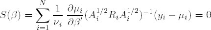
The GEE methodology is based on solving the equations

in which the marginal covariance matrix Vi has been decomposed in the form Ai1/2 Ri Ai1/2, with Ai the matrix with the marginal variances on the main diagonal and zeros elsewhere, and with Ri=Ri(α) the marginal correlation matrix, often referred to as the working correlation matrix. Usually, the marginal covariance matrix Vi=Ai1/2 Ri Ai1/2 contains a vector α of unknown parameters which is replaced for practical purposes by a consistent estimate.
Assuming that the marginal mean μi has been correctly specified as h(μi)=Xiβ, it can be shown that, under mild regularity conditions, the estimator ![]() obtained from solving (12.6.3) is asymptotically normally distributed with mean β and with covariance matrix
obtained from solving (12.6.3) is asymptotically normally distributed with mean β and with covariance matrix
where
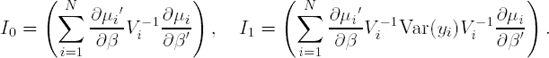
In practice, Var(Yi) in (12.6.4) is replaced by (Yi−μi)(Yi−μi)′, which is unbiased on the sole condition that the mean was again correctly specified.
Note that valid inferences can now be obtained for the mean structure, only assuming that the model assumptions with respect to the first-order moments are correct.
Liang and Zeger (1986) proposed moment-based estimates for the working correlation. To this end, first define deviations:
and decompose the variance slightly more generally as above in the following way:
where φ is an overdispersion parameter.
12.6.1.2. Weighted Generalized Estimating Equations
As stated before, GEE is valid under MCAR. To accommodate MAR missigness, Robins, Rotnitzky, and Zhao (1995) proposed a class of weighted estimating equations. The idea of WGEE is to weight each subject's measurements in the GEEs by the inverse probability that a subject drops out at that particular measurement occasion. This can be calculated as

In the weighted GEE approach, which is proposed to reduce possible bias of ![]() , the score equations to be solved when taking into account the correlation structure are:
, the score equations to be solved when taking into account the correlation structure are:
or

where Yi(d) and μi(d) are the first d−1 elements of Yi and μi respectively. We define ![]() and (Ai1/2
Ri
Ai1/2)−1(d) analogously, in line with the definition of Robins, Rotnitzky and Zhao (1995).
and (Ai1/2
Ri
Ai1/2)−1(d) analogously, in line with the definition of Robins, Rotnitzky and Zhao (1995).
12.6.1.3. A Method Based on Linearization
Both versions of GEE studied sofar can be seen as deriving from the score equations of corresponding likelihood methods. In a sense, GEE result from considering only a subvector of the full vector of scores, corresponding to either the first moments only (the outcomes themselves), or the first and second moments (outcomes and cross-products thereof). On the other hand, they can be seen as an extension of the quasi-likelihood principles, where appropriate modifications are made to the scores to be sufficiently flexible and "work" at the same time. A classical modification is the inclusion of an overdispersion parameter, while in GEE also (nuisance) correlation parameters are introduced.
An alternative approach consists of linearizing the outcome, in the sense of Nelder and Wedderburn (1972), to construct a working variate, to which then weighted least squares is applied. In other words, iteratively reweighted least squares (IRLS) can be used (McCullagh and Nelder, 1989). Within each step, the approximation produces all elements typically encountered in a multivariate normal model, and hence corresponding software tools can be used. In case our models would contain random effects as well, the core of the IRLS could be approached using linear mixed models tools.
Write the outcome vector in a classical (multivariate) generalized linear models fashion:
where, as usual, μi = E(Yi) is the systematic component and εi is the random component, typically following a multinomial distribution. We assume that Var(Yi) =Var(εi) = Σi. The model is further specified by assuming
where ηi is the usual set of linear predictors, g(·) is a vector link function, typically made up of logit components, Xi is a design matrix and β are the regression parameters.
Estimation proceeds by iteratively solving
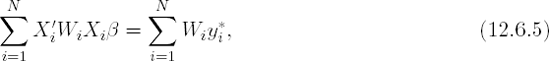
where a working variate Yi* has been defined, following from a first-order Taylor series expansion of ηi around μi:
The weights in (12.6.5) are specified as
In these equations ![]() and
and ![]() are evaluated at the current iteration step. Note that in the specific case of an identity link, ηi = μi, Fi = Ini and Yi = Yi*, whence a standard multivariate regression follows.
are evaluated at the current iteration step. Note that in the specific case of an identity link, ηi = μi, Fi = Ini and Yi = Yi*, whence a standard multivariate regression follows.
The linearization based method can be implemented using the %GLIMMIX macro and PROC GLIMMIX, by ensuring no random effects are included. Empirically corrected standard errors can be obtained by including the EMPIRICAL option.
12.6.2. Random-Effects Models
Models with subject-specific parameters are differentiated from population-averaged models by the inclusion of parameters which are specific to the cluster. Unlike for correlated Gaussian outcomes, the parameters of the random-effects and population-averaged models for correlated binary data describe different types of effects of the covariates on the response probabilities (Neuhaus, 1992).
The choice between population-averaged and random-effects strategies should heavily depend on the scientific goals. Population-averaged models evaluate the overall risk as a function of covariates. With a subject-specific approach, the response rates are modeled as a function of covariates and parameters, specific to a subject. In such models, interpretation of fixed-effects parameters is conditional on a constant level of the random-effects parameter. Population-averaged comparisons, on the other hand, make no use of within-cluster comparisons for cluster-varying covariates and are therefore not useful to assess within-subject effects (Neuhaus, Kalbfleisch and Hauck, 1991).
Whereas the linear mixed model is unequivocally the most popular choice in the case of normally distributed response variables, there are more options in the case of non-normal outcomes. Stiratelli, Laird and Ware (1984) assume the parameter vector to be normally distributed. This idea has been carried further in the work on so-called generalized linear mixed models (Breslow and Clayton, 1993) which is closely related to linear and non-linear mixed models. Alternatively, Skellam (1948) introduced the beta-binomial model, in which the response probability of any response of a particular subject comes from a beta distribution. Hence, this model can also be viewed as a random-effects model. We will consider generalized linear mixed models.
12.6.2.1. Generalized Linear Mixed Models
Perhaps the most commonly encountered subject-specific (or random-effects) model is the generalized linear mixed model. A general framework for mixed-effects models can be expressed as follows.
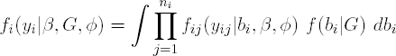
As before, Yij, is the jth outcome measured for cluster (subject) i, i=1, ..., N, j=1, ..., ni and Yi is the ni-dimensional vector of all measurements available for cluster i. It is assumed that, conditionally on q-dimensional random effects bi, assumed to be drawn independently from the N(0, D), the outcomes Yij are independent with densities of the form
with η(μij)= η(E(Yij | bi))=xij′β + zij′bi for a known link function η(·), with xij and zij p-dimensional and q-dimensional vectors of known covariate values, with β a p-dimensional vector of unknown fixed regression coefficients, with φ a scale parameter, and with θij the natural (or canonical) parameter. Further, let f(bi | G) be the density of the N(0, G) distribution for the random effects bi.
Due to the above independence assumption, this model is often referred to as a conditional independence model. This assumption is the basis of the implementation in the NLMIXED procedure. Just as in the linear mixed model case, the model can be extended with residual correlation, in addition to the one induced by the random effects. Such an extended model has been implemented in the SAS GLIMMIX procedure, and its predecessor the %GLIMMIX macro. This advantage is counterbalanced by bias induced by the optimization routine employed by GLIMMIX. It is important to realize that GLIMMIX can be used without random effects as well, thus effectively producing a marginal model, with estimates and standard errors similar to the ones obtained with GEE.
Note: The GLIMMIX procedure is experimental in SAS 9.1. There are advantages to using both PROC GLIMMIX and the %GLIMMIX macro, as we shall see.
In general, unless a fully Bayesian approach is followed, inference is based on the marginal model for Yi which is obtained from integrating out the random effects. The likelihood contribution of subject i then becomes
from which the likelihood for β, D, and φ is derived as
The key problem in maximizing the obtained likelihood is the presence of N integrals over the q-dimensional random effects. In some special cases, these integrals can be worked out analytically. However, since no analytic expressions are available for these integrals, numerical approximation are needed. Here, we will focus on the most frequently used methods to do so. In general, the numerical approximations can be subdivided in those that are based on the approximation of the integrand, those based on an approximation of the data, and those that are based on the approximation of the integral itself. An extensive overview of the currently available approximations can be found in Tuerlinckx et al. (2004), Pinheiro and Bates (2000), and Skrondal and Rabe-Hesketh (2004). Finally, in order to simplify notation, it will be assumed that natural link functions are used, but straightforward extensions can be applied.
When integrands are approximated, the goal is to obtain a tractable integral such that closed-form expressions can be obtained, making the numerical maximization of the approximated likelihood feasible. Several methods have been proposed, but basically all come down to Laplace-type approximations of the function to be integrated (Tierney and Kadane, 1986).
A second class of approaches is based on a decomposition of the data into the mean and an appropriate error term, with a Taylor series expansion of the mean which is a non-linear function of the linear predictor. All methods in this class differ in the order of the Taylor approximation and/or the point around which the approximation is expanded. More specifically, one considers the decomposition
in which h(·) equals the inverse link function η−1(·), and where the error terms have the appropriate distribution with variance equal to Var(Yij|bi) = φ v(μij) for v(·) the usual variance function in the exponential family. Note that, with the natural link function,
Several approximations of the mean μij in (12.6.9) can be considered. One possibility is to consider a linear Taylor expansion of (12.6.9) around current estimates ![]() and
and ![]() i of the fixed effects and random effects, respectively. This will result in the expression
i of the fixed effects and random effects, respectively. This will result in the expression
with Ŵi equal to the diagonal matrix with diagonal entries equal to v(![]() , and for εi* equal to Ŵi−1εi, which still has mean zero. Note that (12.6.10) can be viewed as a linear mixed model for the pseudo data Yi*, with fixed effects β, random effects bi;, and error terms εi*.
, and for εi* equal to Ŵi−1εi, which still has mean zero. Note that (12.6.10) can be viewed as a linear mixed model for the pseudo data Yi*, with fixed effects β, random effects bi;, and error terms εi*.
This immediately yields an algorithm for fitting the original generalized linear mixed model. Given starting values for the parameters β, G and φ in the marginal likelihood, empirical Bayes estimates are calculated for bi, and pseudo data Yi* are computed. Then, the approximate linear mixed model (12.6.10) is fitted, yielding updated estimates for β, G and φ. These are then used to update the pseudo data and this whole scheme is iterated until convergence is reached.
The resulting estimates are called penalized quasi-likelihood estimates (PQL) in the literature (e.g., Molenberghs and Verbeke 2005), or pseudo-quasi-likelihood in the GLIMMIX documentation because they can be obtained from optimizing a quasi-likelihood function which only involves first- and second-order conditional moments, augmented with a penalty term on the random effects. The pseudo-likelihood terminology derives from the fact that the estimates are obtained by (restricted) maximum likelihood of the pseudo-response or working variable.
An alternative approximation is very similar to the PQL method, but is based on a linear Taylor expansion of the mean muij in (12.6.9) around the current estimates ![]() for the fixed effects and around bi=0 for the random effects. The resulting estimates are called marginal quasi-likelihood estimates (MQL). See Breslow and Clayton (1993) and Wolfinger and O'Connell (1993) for details. Since the linearizations in the PQL and the MQL methods lead to linear mixed models, the implementation of these procedures is often based on feeding updated pseudo data into software for the fitting of linear mixed models. However, it should be emphasized that outputs that the results from these fittings, which are often reported intermediately, should be interpreted with great care. For example, reported (log-)likelihood values correspond to the assumed normal model for the pseudo data and should not be confused with (log-)likelihood for the generalized linear mixed model for the actual data at hand. Further, fitting of linear mixed models can be based on maximum likelihood (ML) as well as restricted maximum likelihood (REML) estimation. Hence, within the PQL and MQL frameworks, both methods can be used for the fitting of the linear model to the pseudo data, yielding (slightly) different results. Finally, the quasi-likelihood methods discussed here are very similar to the method of linearization discussed in Section 12.6.1 for fitting generalized estimating equations (GEE). The difference is that here, the correlation between repeated measurements is modeled through the inclusion of random effects, conditional on which repeated measures are assumed independent, while, in the GEE approach, this association is modeled through a marginal working correlation matrix.
for the fixed effects and around bi=0 for the random effects. The resulting estimates are called marginal quasi-likelihood estimates (MQL). See Breslow and Clayton (1993) and Wolfinger and O'Connell (1993) for details. Since the linearizations in the PQL and the MQL methods lead to linear mixed models, the implementation of these procedures is often based on feeding updated pseudo data into software for the fitting of linear mixed models. However, it should be emphasized that outputs that the results from these fittings, which are often reported intermediately, should be interpreted with great care. For example, reported (log-)likelihood values correspond to the assumed normal model for the pseudo data and should not be confused with (log-)likelihood for the generalized linear mixed model for the actual data at hand. Further, fitting of linear mixed models can be based on maximum likelihood (ML) as well as restricted maximum likelihood (REML) estimation. Hence, within the PQL and MQL frameworks, both methods can be used for the fitting of the linear model to the pseudo data, yielding (slightly) different results. Finally, the quasi-likelihood methods discussed here are very similar to the method of linearization discussed in Section 12.6.1 for fitting generalized estimating equations (GEE). The difference is that here, the correlation between repeated measurements is modeled through the inclusion of random effects, conditional on which repeated measures are assumed independent, while, in the GEE approach, this association is modeled through a marginal working correlation matrix.
Note that, when there are no random effects, both this method and GEE reduce to a marginal model, the difference being in the way the correlation parameters are estimated. In both cases, it is possible to allow for misspecification of the association structure by resorting to empirically corrected standard errors. When this is done, the methods are valid under MCAR. In case we would have confidence in the specified correlation structure, purely model-based inference can be conducted and hence the methods are valid when missing data are MAR.
A third method of numerical approximation is based on the approximation of the integral itself. Especially in cases where the above two approximation methods fail, this numerical integration proofs to be very useful. Of course, a wide toolkit of numerical integration tools, available from the optimization literature, can be applied. Several of those have been implemented in various software tools for generalized linear mixed models. A general class of quadrature rules selects a set of abscissas and constructs a weighted sum of function evaluations over those. In the particular context of random-effects models, so-called quadrature rules can be used (Pinheiro and Bates 1995, 2000), where the numerical integration is centered around the EB estimates of the random effects, and the number of quadrature points is then selected in terms of the desired accuracy.
To illustrate the main ideas, we consider Gaussian and adaptive Gaussian quadrature, designed for the approximation of integrals of the form ∫ f(z) φ(z) dz, for an known function f (z)and forφ(z) the density of the (multivariate) standard normal distribution. We will first standardize the random effects such that they get the identity covariance matrix. Let δi be equal to δi = G−1/2 bi. We then have that δi is normally distributed with mean 0 and covariance I. The linear predictor then becomes θij = xij′β + zij′ G1/2 δi, so the variance components in G have been moved to the linear predictor. The likelihood contribution for subject i then equals

Obviously, (12.6.11) is of the form ∫ f(z) φ(z) dz as required to apply (adaptive) Gaussian quadrature.
In Gaussian quadrature, ∫ f (z) φ(z) dz is approximated by the weighted sum
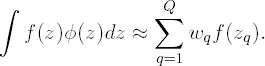
Q is the order of the approximation. The higher Q the more accurate the approximation will be. Further, the so-called nodes (or quadrature points) zq are solutions to the Qth order Hermite polynomial, while the wq are well-chosen weights. The nodes zq and weights wq are reported in tables. Alternatively, an algorithm is available for calculating all zq and wq for any value Q (Press et al, 1992).
Figure 12-5. Graphical illustration of Gaussian (left panel) and adaptive Gaussian (right panel) quadrature. The triangles indicate the position of the quadrature points, while the rectangles indicate the contribution of each point to the integral.

In case of univariate integration, the approximation consists of subdividing the integration region in intervals, and approximating the surface under the integrand by the sum of surfaces of the so-obtained approximating rectangles. An example is given in the left panel of Figure 12.5, for the case of Q=10 quadrature points. A similar interpretation is possible for the approximation of multivariate integrals. Note that the figure immediately highlights one of the main disadvantages of (non-adaptive) Gaussian quadrature, i.e., the fact that the quadrature points zq are chosen based on φ(z), independent of the function f(z) in the integrand. Depending on the support of f(z), the zq will or will not lie in the region of interest. Indeed, the quadrature points are selected to perform well in case f(z) φ(z) approximately behaves like φ(z), i.e., like a standard normal density function. This will be the case, for example, if f(z) is a polynomial of a sufficiently low order. In our applications however, the function f(z) will take the form of a density from the exponential family, hence an exponential function. It may then be helpful to rescale and shift the quadrature points such that more quadrature points lie in the region of interest. This is shown in the right panel of Figure 12.5, and is called adaptive Gaussian quadrature.
In general, the higher the order Q, the better the approximation will be of the N integrals in the likelihood. Typically, adaptive Gaussian quadrature needs (much) less quadrature points than classical Gaussian quadrature. On the other hand, adaptive Gaussian quadrature requires for each unit the numerical maximization of a function of the form (f(z)φ(z)) for the calculation of ![]() . This implies that adaptive Gaussian quadrature is much more time consuming.
. This implies that adaptive Gaussian quadrature is much more time consuming.
Since fitting of generalized linear mixed models is based on maximum likelihood principles, inferences for the parameters are readily obtained from classical maximum likelihood theory.
12.6.3. Marginal versus Random-Effects Models
Note that there is an important difference with respect to the interpretation of the fixed effects β. Under the classical linear mixed model (Verbeke and Molenberghs, 2000), we have that E(Yi) equals Xiβ, such that the fixed effects have a subject-specific as well as a population-averaged interpretation. Under non-linear mixed models, however, this does no longer hold in general. The fixed effects now only reflect the conditional effect of covariates, and the marginal effect is not easily obtained anymore as E(Yi) is given by
However, in a biopharmaceutical context, we is often primarily interested in hypothesis testing, and the random-effects framework can be used to this effect.
Note that both WGEE and GLMM are valid under MAR, at the extra condition that the model for weights in WGEE has been specified correctly. Nevertheless, the parameter estimates between both are rather different. This is due to the fact that GEE and WGEE parameters have a marginal interpretation, describing average longitudinal profiles, whereas GLMM parameters describe a longitudinal profile, conditional upon the value of the random effects. Let us now provide an overview of the differences between marginal and random-effects models for non-Gaussian outcomes (a detailed discussion can be found in Molenberghs and Verbeke (2004). The interpretation of the parameters in both types of model (marginal or random-effects) is completely different.
Figure 12-6. Representation of model families and corresponding inference (M stands for marginal and RE stands for random-effects). A parameter between quotes indicates that marginal functions but no direct marginal parameters are obtained, since they result from integrating out the random effects from the fitted hierarchical model.

A schematic display is given in Figure 12.6. Depending on the model family (marginal or random-effects), we are led to either marginal or hierarchical inference. It is important to realize that in the general case the parameter βM resulting from a marginal model is different from the parameter βRE even when the latter is estimated using marginal inference. Some of the confusion surrounding this issue may result from the equality of these parameters in the very special linear mixed model case. When a random-effects model is considered, the marginal mean profile can be derived, but it will generally not produce a simple parametric form. In Figure 12.6 this is indicated by putting the corresponding parameter between quotation marks.
12.6.4. Analysis of Depression Trial Data
Let us now analyze the clinical depression trial, introduced in Section 12.2. The binary outcome of interest is the YBIN variable (it is equal to 1 if the HAMD17 score is larger than 7, and 0 otherwise). The primary null hypothesis has been tested using both GEE and WGEE (with PROC GENMOD), as well as GLMM with adaptive and non-adaptive Gaussian quadrature (with PROC NLMIXED) in Dmitrienko et al. (2005, Chapter 5). Now, we will test the hypothesis using GEE based on linearization, as well as GLMM based on the penalized quasi-likelihood method. Both methods can be fitted using the GLIMMIX macro. Beginning with SAS 9.1, there is an experimental GLIMMIX procedure, which can be used as well. We include the fixed categorical effects of treatment, visit, and treatment-by-visit interaction, as well as the continuous, fixed covariates of baseline score and baseline score-by-visit interaction. A random intercept will be included when considering the random-effect models.
12.6.4.1. %GLIMMIX Macro for the Marginal Model
We will consider the marginal model:
where Xi is the design matrix for subject i, containing all covariates and an intercept.
Program 12.1 fits Model (12.6.12) with exchangeable working assumptions using the %GLIMMIX macro. The macro is based on fitting the iterative procedure, outlined in Section 12.6.1. The Generalized Linear Models shell linearizes the outcome and computes the weights, as in (12.6.6) and (12.6.7). Specific statements that govern this procedure are the ERROR and LINK statement. We chose the binomial error structure. The logit link is the default for this option, but we have still chosen to specify it, for clarity. The procedure is based on the MIXED procedure, used to solve iteratively reweighted least squares equations (12.6.5). Virtually all statements, available in the MIXED procedure can be used. They are passed on, in string form, to the macro via the STMTS option. Note that TYPE=CS, referring to compound symmetry, must be used here. For unstructured working assumptions, we use TYPE=UN, for AR(1) this would be TYPE=AR(1), and for independence assumptions, TYPE=SIMPLE needs to be used. One set of assumptions, those corresponding to the PROC MIXED statement, are passed on via a separate statement, i.e., the PROCOPT string. Note that we have inserted the EMPIRICAL option, to ensure the empirically corrected standard errors are produced. Omitting the EMPIRICAL option produces the model-based standard errors. We have a choice between the updating methods that are available in the MIXED procedure.
To receive the output that would be produced by the MIXED procedure, one can use OPTIONS=MIXPRINTLAST within the STMTS option. To study the PROC MIXED output at each, we add the MIXPRINTALL option. Arguably, the latter is primarily useful for debugging purposes.
Example 12-1. %GLIMMIX macro for the linearization-based method in the depression trial example
%glimmix(data=depression, procopt=%str(method=ml empirical),
    stmts=%str(
        class patient visit trt;
        model ybin = visit trt*visit basval basval*visit / solution;
        repeated visit / subject=patient type=cs rcorr;
        ),
    error=binomial,
link=logit); |
The typical GLIMMIX output consists of tables copied from the MIXED output, as well as some additional information. Typical output includes bookkeeping information such as model information, dimensions, number of observations. Since we included the RCORR option in the REPEATED statement, the fitted correlation matrix of the measurements is given, which is to be interpreted as the working correlation matrix. In our case, this is a 5 × 5 correlation matrix with off-diagonal elements equal to 0.3317, the exchangeable working correlation. Output 12.1, the panel Covariance Parameter Estimates portion of the output, must be interpreted with caution, though, for reason that we will explain.
Example. Output from Program 12.1. Covariance Parameter Estimates.
Covariance Parameter Estimates Cov Parm Subject Estimate CS PATIENT 0.3140 Residual 0.6326 |
The working correlation is obtained from the usual compound-symmetry equation:
In the following output, the residual value is copied as the extra-dispersion parameter:
Example. Output from Program 12.1. GLIMMIX Model Statistics.
GLIMMIX Model Statistics Description Value Deviance 746.6479 Scaled Deviance 1180.3240 Pearson Chi-Square 673.9938 Scaled Pearson Chi-Square 1065.4703 Extra-Dispersion Scale 0.6326 |
It is best not to use this portion of output, since it is not appropriately adapted to the combination of generalized linear model and the repeated measures nature of the data. In case we had used independence working assumptions, there would be a single covariance parameter only, which could then be considered the overdispersion parameter. Arguably, there is little basis to do so, and it is unlikely to see almost no overdispersion with independence and strong underdispersion with exchangeability. It might make more sense to consider the total variance in the exchangeable case, i.e., 0.3140+0.6326, the overdispersion parameter. Similarly, it would be better to ignore the fit statistics portion of output, copied from the MIXED procedure.
The most relevant portion of the output is the Solution for Fixed Effects table, with its associated F tests.
Example. Output from Program 12.1. Solution and Type 3 Tests for Fixed Effects.
Solution for Fixed Effects

              Visit                      Standard
Effect        Number  TRT    Estimate     Error      DF   t Value  Pr > |t|

Intercept                     −1.2326    0.7853     168     −1.57    0.1184
VISIT         4                0.4457    1.2147     517      0.37    0.7138
...
VISIT*TRT     8       1       −0.6942    0.3810     517     −1.82    0.0690
...
BASVAL*VISIT  7               0.02439   0.05170     517      0.47    0.6373
BASVAL*VISIT  8                     0         .       .       .       .

Type 3 Tests of Fixed Effects

                 Num     Den
Effect            DF      DF    F Value    Pr > F

VISIT              4     517       0.39    0.8128
VISIT*TRT          5     517       1.22    0.3000
BASVAL             1     168      22.17    <.0001
BASVAL*VISIT 4 517 1.79 0.1291 |
These estimates, with both model-based and empirically corrected standard errors, are given in the linearization column of Table 12.2, next to the estimates for GEE and WGEE. Clearly, the estimates under exchangeability for the linearization-based method are very similar to those for GEE. Since we did not include the treatment as a main effect, the output immediately produces the treatment effects at the different time points. For instance, the estimate of the effect of treatment at the endpoint is −0.6942, with corresponding p value equal to 0.0690. Comparing this with the result of GEE (p-value of treatment effect at the last visit is 0.0633), it is clear that both are very similar. However, when performing a WGEE analysis is performed, the result of this contrast changes a lot (p-value is 0.0325).
12.6.4.2. PROC GLIMMIX for the Marginal Model
We can also use PROC GLIMMIX to fit models of a marginal type, subject-specific type, as well as models with subject-specific effects and residual association in addition to that. Program 12.2 relies on PROC GLIMMIX to fit a model identical to the model fitted by Program 12.1. Even though Program 12.2 is rather different, at first sight, from Program 12.1, the correspondence is almost immediate. Again, users of PROC MIXED for linear mixed models will recognize that the code here is very similar to that used in PROC MIXED. The reason is that, internally, PROC GLIMMIX calls PROC MIXED each time a linear mixed model needs to be fitted to newly updated pseudo data.
| GEE | WGEE | Linearization | ||||
|---|---|---|---|---|---|---|
| intercept | −1.22 | (0.77;0.79) | −0.70 | (0.64;0.86) | −1.23 | (0.75;0.79) |
| visit 4 | 0.43 | (1.05;1.22) | −0.08 | (0.88;1.85) | 0.45 | (1.05;1.22) |
| visit 5 | −0.48 | (0.91;1.23) | −0.13 | (0.70;1.55) | −0.47 | (0.92;1.23) |
| visit 6 | 0.06 | (0.86;1.03) | 0.19 | (0.72;1.14) | 0.05 | (0.86;1.03) |
| visit 7 | −0.25 | (0.89;0.91) | −0.28 | (0.82;0.88) | −0.25 | (0.89;0.91) |
| trt × visit 4 | −0.24 | (0.54;0.57) | −1.57 | (0.41;0.99) | −0.22 | (0.53;0.56) |
| trt × visit 5 | −0.09 | (0.39;0.40) | −0.67 | (0.21;0.65) | −0.08 | (0.38;0.40) |
| trt × visit 6 | 0.17 | (0.34;0.35) | 0.62 | (0.23;0.56) | 0.18 | (0.34;0.35) |
| trt × visit 7 | −0.43 | (0.36;0.35) | 0.57 | (0.30;0.37) | −0.42 | (0.35;0.35) |
| trt × visit 8 | −0.71 | (0.38;0.38) | −0.84 | (0.32;0.39) | −0.69 | (0.37;0.38) |
| baseline | 0.08 | (0.04;0.04) | 0.07 | (0.03;0.05) | 0.08 | (0.04;0.04) |
| baseline × visit 4 | 0.12 | (0.07;0.07) | 0.24 | (0.06;0.13) | 0.12 | (0.06;0.07) |
| baseline × visit 5 | 0.09 | (0.05;0.07) | 0.07 | (0.04;0.08) | 0.09 | (0.05;0.07) |
| baseline × visit 6 | 0.01 | (0.05;0.05) | 0.01 | (0.04;0.06) | 0.01 | (0.05;0.88) |
| baseline × visit 7 | 0.02 | (0.05;0.05) | 0.03 | (0.05;0.05) | 0.02 | (0.05;0.05) |
Example 12-2. PROC GLIMMIX for the linearization-based method in the depression trial example
proc glimmix data=depression method=rspl empirical;
    class patient visit trt;
    model ybin (event='1')=visit trt*visit basval basval*visit/dist=binary solution;
    random _residual_/subject=patient type=cs;
run; |
The most important option in PROC GLIMMIX is METHOD. In Program 12.2, METHOD=RSPL specifies the PQL method based on REML for the linear mixed models. Note that, strictly speaking, the "penalized" part of PQL is absent, since there are no random effects and hence no random-effects penalty. In this case, it is more straightforward to think of restricted pseudo-likelihood (RPL). An overview of the other available options is given in Table 12.3.
| GLIMMIX option | Quasi-likelihood type PQL/MQL | Inference pseudo-data GLIMMIX option ML/REML |
|---|---|---|
| METHOD=RSPL | PQL | REML |
| METHOD=MSPL | PQL | ML |
| METHOD=RMPL | MQL | REML |
| METHOD=MMPL | MQL | ML |
The CLASS statement in PROC GLIMMIX specifies which variables should be considered as factors. Such classification variables can be either character or numeric. Internally, each of these factors will correspond to a set of dummy variables.
The MODEL statement names the response variable and all fixed effects, which determine the Xi matrices. By default, an intercept is added. The EVENT option (EVENT='1') specifies that the probability to be modeled is P(Yij = 1) (the probability of a severe infection) rather than P(Yij = 0). The SOLUTION option is used to request the printing of the estimates for all the fixed effects in the model, together with standard errors, t-statistics, corresponding p-values and confidence intervals. The DIST option is used to specify the conditional distribution of the data, given the random effects. Various distributions are available, including the normal, Bernoulli, Binomial,and Poisson distribution. In Program 12.2, the Bernoulli distribution is specified (DIST=BINARY). The default link function is the natural link (in this example, it is the logit link).
The REPEATED statement of the %GLIMMIX macro corresponds to the RANDOM=_residual_ statement in PROC GLIMMIX. SAS refers to this as the R-side of the random statement. It is useful to think of it as the variance-covariance matrix of the outcome vector Yi, of which the variances follow from the mean-variance link, but the correlation structure needs to be specified (as in GEE). When random effects are present, this structure refers to the residual correlation, in addition to the correlation induced by the random effects. Changing the TYPE option in the RANDOM statement to SIMPLE, CS or UN, respectively, combined with either omission or inclusion of the EMPIRICAL option in PROC GLIMMIX produces exactly the same results as with the %GLIMMIX macro, i.e., the results reported in the third panel of Table 12.2.
The output form PROC GLIMMIX in Program 12.2, although structured differently from the %GLIMMIX macro output, is largely equivalent. The fact that the empirically corrected standard errors are produced is properly acknowledged:
Example. Output of Program 12.2. Part of the Model Information.
The GLIMMIX Procedure

                 Model Information

Fixed Effects SE Adjustment Sandwich - Classical |
The fact that a marginal model (i.e., a model without random effects) is used is acknowledged through reference to the so-called R-side covariance parameters:
Example. Output of Program 12.2. Part of the Dimensions.
Dimensions R-side Cov. Parameters 2 |
PROC GLIMMIX in Program 12.2 took 11 iterations to converge. The final covariance parameters are equivalent to the ones produced by the %GLIMMIX macro:
Example. Output of Program 12.2. Covariance Parameter Estimates.
Covariance Parameter Estimates

                                   Standard
Cov Parm    Subject    Estimate       Error

CS          PATIENT      0.3196     0.05209
Residual 0.6469 0.03955 |
PROC GLIMMIX also produces the fixed-effects parameters (again equivalent, up to numerical accuracy, to their %GLIMMIX macro counterparts) together with associated F tests.
Example. Output from Program 12.2. Solution and Type 3 Tests for Fixed Effects.
Solutions for Fixed Effects

              Visit                    Standard
Effect        Number  TRT    Estimate     Error     DF    t Value  Pr > |t|

Intercept                     −1.2331    0.7852    168      −1.57    0.1182
VISIT         4                0.4463    1.2146    517       0.37    0.7134
...
VISIT*TRT     8       1       −0.6939    0.3810    517      −1.82    0.0691
...
BASVAL*VISIT  7               0.02440   0.05170    517       0.47    0.6372
BASVAL*VISIT  8                     0         .      .        .       .

Type III Tests of Fixed Effects

                 Num      Den
Effect            DF       DF    F Value    Pr > F

VISIT              4      517       0.39    0.8129
VISIT*TRT          5      517       1.22    0.3003
BASVAL             1      168      22.18    <.0001
BASVAL*VISIT 4 517 1.79 0.1293 |
Again as long as PROC GLIMMIX is experimental (as in SAS 9.1), it is a good idea to use the %GLIMMIX macro as well. Also, having the macro as a backup may increase program's chances to reaching convergence.
12.6.4.3. PROC GLIMMIX for the Random-Effects Model
PROC GLIMMIX supports the marginal and penalized quasi-likelihood methods. We will fit the following random-effects model, using the PQL method: assume that, conditional on subject-specific random intercepts, bi, Yij is Bernoulli distributed with mean πij, modeled as
in which Xi is the design matrix with covariates described above, β is the vector of fixed effects parameters, Zi is a design matrix for the random effects (in this case a row of ones), and bi is the random intercept assumed to be normally distributed with mean 0 and variance d.
The procedure has many more statements and options than those presented here, but we restrict to the basic statements needed to fit a generalized linear mixed model.
Program 12.3 fits this random-effects using PQL based on REML estimation for the linear mixed models for the pseudo data.
Example 12-3. PROC GLIMMIX for the random-effects model using PQL maximization in the depression trial example
proc glimmix data=depression method=rspl;
    class patient visit trt;
    model ybin (event='1')=visit trt*visit basval basval*visit/dist=binary solution;
    random intercept/subject=patient;
run; |
Most of the statements used in Program 12.3 were described above, except for the RANDOM statement. The RANDOM statement defines the random effects in the model, i.e., the Zi matrices containing the covariates with subject-specific regression coefficients. Note that when random intercepts are required (as in this example), this requirement should be specified explicitly, which is in contrast to the MODEL statement where an intercept is included by default. The SUBJECT option identifies the subjects in the DEPRESSION data set. The variable in the SUBJECT option can be continuous or categorical (specified in the CLASS statement); however, when it is continuous, PROC GLIMMIX considers a record to be from a new subject whenever the value of this variable is different from the previous record.
Suppose that random slopes for the time trend were to be included as well. This can be achieved by replacing the RANDOM statement in Program 12.3
random intercept time/subject=patient type=un;
    run;
Here TYPE=UN specifies that the random-effects covariance matrix G is a general unstructured 2 × 2 matrix. Special structures are available, e.g., equal variance for the intercepts and slopes, or independent intercepts and slopes.
The output of Program 12.3 includes information about the fitted model and the estimation procedure. The Residual PL estimation technique refers to PQL with REML (restricted or residual maximum likelihood) for the fitting of the linear models for the pseudo data:
Example. Output of Program 12.3. Model Information.
The GLIMMIX Procedure

              Model Information

Data Set                      WORK.DEPRESSION
Response Variable             ybin
Response Distribution         Binary
Link Function                 Logit
Variance Function             Default
Variance Matrix Blocked By    PATIENT
Estimation Technique          Residual PL
Degrees of Freedom Method Containment |
The Fit Statistics portion of the output gives minus twice the residual log-pseudo-likelihood value evaluated in the final solution, together with the information criteria of Akaike (AIC) and Schwarz (BIC), as well as a finite-sample corrected version of AIC (AICC). When REML estimation is used for the fitting of the linear mixed models for the pseudo data, an objective function is maximized which is called residual log-likelihood function, while, strictly speaking, the function is not a log-likelihood, and should not be used as a log-likelihood. We refer to Verbeke and Molenberghs (2000, Chapters 5 and 6) for a more detailed discussion with examples. Further, information criteria are statistics that are sometimes used to compare non-nested models which cannot be compared based on a formal testing procedure. The main idea behind information criteria is to compared models based on their maximized (residual) log-likelihood value (or equivalently minimized minus twice the log-likelihood value), while at the same time penalizing for including an excessive number of. They should by no means be interpreted as formal statistical tests of significance. In specific examples, different information criteria can even lead to different model selections. An example of this is given in Section 6.4 of Verbeke and Molenberghs (2000) in the context of linear mixed models. More details about the use of information criteria can be found in Akaike (1974), Schwarz (1978), and Burnham and Anderson (1998).
Example. Output of Program 12.3. Fit Statistics and Covariance Parameter Estimates.
Fit Statistics

-2 Res Log Pseudo-Likelihood        3488.65
Pseudo-AIC  (smaller is better)     3490.65
Pseudo-AICC (smaller is better)     3490.65
Pseudo-BIC  (smaller is better)     3493.78
Pseudo-CAIC (smaller is better)     3494.78
Pseudo-HQIC (smaller is better)     3491.92
Pearson Chi-Square                   400.28
Pearson Chi-Square / DF                0.58

       Covariance Parameter Estimates

                                    Standard
Cov Parm     Subject    Estimate       Error

Intercept PATIENT 2.5318 0.5343 |
Next, Output 12.3 presents two tables containing estimates and inferences for the fixed effects in the model. The reported inferences immediately result from the linear mixed model fitted to the pseudo data in the last step of the iterative estimation procedure. From the output, it is immediately clear the treatment effect at the last visit is clearly insignificant (p-value is 0.1286). Comparing this with the p-value obtained after fitting GLMM with adaptive Gaussian quadrature (p = 0.0954), we see that both yield an insignificant effect.
Example. Output of Program 12.3. Solutions and Type 3 Tests of Fixed Effects.
Solutions for Fixed Effects

              Visit                       Standard
Effect        Number  TRT    Estimate      Error      DF   t Value   Pr > |t|

Intercept                     −1.7036     1.0607     167     −1.61     0.1101
...
VISIT*TRT     8       1       −0.8426     0.5537     518     −1.52     0.1286
...
BASVAL*VISIT  7               0.02743    0.06897     518      0.40     0.6911
BASVAL*VISIT  8                     0          .       .       .        .

Type III Tests of Fixed Effects

                 Num      Den
Effect            DF       DF    F Value    Pr > F

VISIT              4      518       0.27    0.8959
VISIT*TRT          5      518       0.85    0.5141
BASVAL             1      518      18.12    <.0001
BASVAL*VISIT 4 518 1.20 0.3115 |
The Covariance Parameter Estimates portion of the output lists estimates and associated standard errors for the variance components in the model, i.e., for the elements in the random-effects covariance matrix G. In our example, this is the random-intercepts variance g.
Table 12.4 compares the parameter estimates and standard errors with the results obtained by fitting GLMM with adaptive Gaussian quadrature, using PROC NLMIXED. Obviously, there are some differences between these two methods for certain parameters. Since both approaches are likelihood-based, validity under the MAR assumption should be fulfilled. For PROC NLMIXED, the integral is approximated using adaptive Gaussian quadrature, which is quite an accurate method, if a sufficient number of quadrature points are chosen. However, PROC GLIMMIX (or %GLIMMIX macro) is based on penalized quasi-likelihood, and thus the mean is approximated by a Taylor expansion. This approximation can be relatively poor for random-effects models and hence results thereof should be treated with caution.
| PQL | AGQ | |||
|---|---|---|---|---|
| intercept | −1.70 | (1.06) | −2.31 | (1.34) |
| visit 4 | 0.66 | (1.48) | 0.64 | (1.75) |
| visit 5 | −0.44 | (1.29) | −0.78 | (1.51) |
| visit 6 | 0.17 | (1.22) | 0.19 | (1.41) |
| visit 7 | −0.23 | (1.25) | −0.27 | (1.43) |
| treatment × visit 4 | −0.29 | (0.66) | −0.54 | (0.82) |
| treatment × visit 5 | −0.10 | (0.53) | −0.20 | (0.68) |
| treatment × visit 6 | 0.33 | (0.49) | 0.41 | (0.64) |
| treatment × visit 7 | −0.47 | (0.52) | −0.68 | (0.67) |
| treatment × visit 8 | −0.84 | (0.55) | −1.20 | (0.72) |
| baseline | 0.10 | (0.06) | 0.15 | (0.07) |
| baseline × visit 4 | 0.14 | (0.09) | 0.21 | (0.11) |
| baseline × visit 5 | 0.12 | (0.07) | 0.17 | (0.09) |
| baseline × visit 6 | 0.007 | (0.07) | 0.01 | (0.08) |
| baseline × visit 7 | 0.03 | (0.07) | 0.03 | (0.08) |
12.6.4.4. GLIMMIX Macro for the Random-Effects Model
Although still experimental in SAS Version 9.1, PROC GLIMMIX can be viewed as a formal procedure that has grown out of the %GLIMMIX macro, applied earlier for fitting generalized estimating equations (GEE) based on linearization. In GEE, the association between repeated measures is modeled through a marginal working correlation matrix. Now, this correlation is modeled via the inclusion of random effects, conditionally on which repeated measures are assumed independent. This similarity implies that the same macro can be used for fitting generalized linear mixed models as well. Without going into much detail, we present in Program 12.4 the SAS code needed to repeat the previous analysis with the %GLIMMIX macro.
Example 12-4. %GLIMMIX macro for the random-effects model using PQL maximization in the depression trial example
%glimmix(
   data=depression,
   stmts=%str(
      class class patient visit trt;
      model ybin = visit trt*visit basval basval*visit/solution;
      random intercept/subject=patient;
      parms (4) (1)/hold=2;
      ),
error=binomial); |
The statements that appear in the STMTS statement are directly fed into the PROC MIXED calls needed for fitting the linear mixed models to the pseudo data. Note that the %GLIMMIX macro by default includes a residual overdispersion parameter. If the corresponding generalized linear mixed model does not contain such a parameter, it should explicitly be kept equal to one by the user. This is done using the HOLD option in the PARMS statement.
Since PROC MIXED uses REML estimation by default, Program 12.4 requests PQL estimation based on REML fitting for the pseudo data. If ML fitting is required, this can be specified by adding the line
procopt=%str(method=ml),
to the GLIMMIX call in Program 12.4. If MQL is required, rather than the default PQL, this can be specified by adding the following line
options=MQL,
Without discussing the output from the %GLIMMIX macro in much detail, we here present some output tables, which can be compared with the output from PROC GLIMMIX (Program 12.3).
Example. Partial Output of Program 12.4
Covariance Parameter Estimates

Cov Parm      Subject    Estimate

Intercept     PATIENT      2.5318
Residual                   1.0000

           Fit Statistics

-2 Res Log Likelihood          3488.6
AIC (smaller is better)        3490.6
AICC (smaller is better)       3490.7
BIC (smaller is better)        3493.8
Solution for Fixed Effects
Visit Standard
Effect Number TRT Estimate Error DF t Value Pr > |t|
Intercept −1.7036 1.0607 167 −1.61 0.1101
...
VISIT*TRT 8 1 −0.8426 0.5537 518 −1.52 0.1286
...
BASVAL*VISIT 7 0.02743 0.06897 518 0.40 0.6911
BASVAL*VISIT 8 0 . . . .
Type 3 Tests of Fixed Effects
Num Den
Effect DF DF F Value Pr > F
VISIT 4 518 0.27 0.8959
VISIT*TRT 5 518 0.85 0.5141
BASVAL 1 518 18.12 <.0001
BASVAL*VISIT 4 518 1.20 0.3115 |
Output 12.4 shows that, indeed, the residual overdispersion parameter was set to one. The obtained results are identical to the results produced by PROC GLIMMIX in Program 12.3.