3.3. Training and Test Set Selection

In order to build reliable and predictive models, care must be taken in selecting training and test sets. When the test set is representative of the training set, one can obtain an accurate estimate of the model's performance. Ideally, if there is sufficient data, the modeler can divide the data into three different data sets: training set, validation set, and test set. The training set is used to train different models. Then each of these models is applied to the validation set and the model with the minimum error is selected as the final model and applied to the test data set to estimate the prediction error of the model. More often than not, there is insufficient data to apply this technique.

Another method used to calculate the model prediction error is cross-validation. In this method, the data are divided into K parts, each approximately the same size. For each of the K parts, the model is trained on the remaining K – 1 parts and then applied to the Kth part and the prediction error calculated. The final estimate of the model prediction error is the average prediction error over all K parts. The biggest question associated with this method is how to choose K. If K is chosen to be equal to the sample size, then the estimate of error will be unbiased, but the variance will be high. As K decreases, the variance decreases but the bias increases, so one needs to find the appropriate trade off between bias and variance. see Hastie, Tibshirani and Friedman (2001) for more information.

Another method which is similar to cross-validation is the bootstrap method. This method takes a bootstrap sample from the original data set and uses the data to train the model. Then, to calculate the model prediction error, the model is applied to either the original data set or to the data not included in the bootstrap sample. This procedure is repeated a large number of times and the final prediction error is the average prediction error over all bootstrap samples. The main issue with this method is whether the original data set is used to calculate the prediction error or only the observations not included in the bootstrap sample. When the original sample is used, the model will give relatively good predictions because the bootstrap sample (training set) is very similar to the original sample (test set). One solution to reduce this bias is to use the "0.632 estimator". For more information on this method see Efron and Tibshirani (1998).

3.3.1. Proposed Procedure for Selecting Training and Test Sets

The methods discussed above are easy to implement and will give adequate estimates of the prediction error provided there are no outlying points in either the response space or the descriptor space. Often in drug discovery data sets there are points of high influence or outliers, so excluding them from the training set is an important consideration. Therefore, we developed a training and test set selection procedure that limits the number of outliers and points of influence in the training set. In this section we provide an overview of the proposed method and apply it to the solubility data set.

Our goal is to develop a training and test set selection algorithm that accomplishes the following goals:

• Select a test set that is representative of the training set.

• Minimize the number of outliers and influential points in the training set.

Suppose a data set contains only one descriptor. Then it would be fairly easy to come up with an algorithm that meets the above goals. For instance, the modeler could use a two dimensional plot to identify outliers and points of influence, assign these to the test set, and then take a random sample of the remaining points and assign them to the training set. To view the data set selection, the modeler could again use a two-dimensional plot and if the test set did not visually appear to be representative of the training set, the modeler could take another random sample.

The above procedure is simple, easy to explain to scientists and accomplishes the two goals when p = 1, but it is not easily extendable for p > 1 because the modeler would have to view two-dimensional projections to identify outliers and points of influence. Furthermore, selecting a representative sample in p + 1-dimensional space would be impossible Unless the following were true: instead of using each descriptor, a summary measure for each observation in the descriptor space was used, for instance, the leverage value of each observation. Recall that the leverage value for the ith observation is the distance between the observation and the center of the descriptor space. By using the leverage values and the responses, we have reduced down to 2 from p + 1 and the algorithm discussed above (when p = 1) could be used to develop an algorithm for training and test set selection.

The basic algorithm for the proposed procedure is defined as follows:

To enhance the above algorithm, the user can select how the bin size is calculated. One option, referred to as the normal bin width, defines the bin width to be:

W = 3.49σN^−1/3,

where N is the number of samples and σ is the standard deviation of either the responses or the leverages. The second option, referred to as robust bin width, defines the bin width to be:

W = 2(IQR)N^−1/3,

where IQR is the interquartile range of either the response or the leverage values and N is defined above. We have found that the robust bin width results in more cells being defined and we suggest the normal bin width be used if the data are sparse. For discussions on the optimal bin size see Scott (1979).

After running the basic algorithm on a number of examples, we added two addition features to improve it. The user has an option of pre-allocating particular observations to either the training or test data sets. The other feature we added allows the user to specify the seed used to initialize the random number generator. This allows the user to get the same results on multiple runs.

3.3.2. TRAINTEST Module

The algorithm described above was implemented in a SAS/IML module (TRAINTEST module) that can be found on the book's web site. There are seven inputs to this module:

• the matrix of descriptors

• the vector of responses

• the type of bins to use (normal or robust)

• the desired proportion of observations in the training set

• a vector indicating the data set each observation should be in (if the user doesn't want to pre-allocate any observations, then this vector should be initialized to a vector of zeros)

• the level of the confidence region around the leverage values and the response

• the seed

(If the seed is set to zero, then the module allows SAS to initialize the random number generator; SAS uses the system time for initialization.)

The TRAINTEST module produces three outputs plus a visual display of the training and test set selections. The three outputs are: a vector indicating the data set each observation belongs to, the vector of leverage values, and the observed proportion of observations in the training set. Finally, the module creates a SAS data set (PLOTINFO) that can be used to create a plot of leverage values versus responses. The PLOTTYPE variable in this data sets serves as a label for individual observations: PLOTTYPE=1 if the observation is in the training set, PLOTTYPE=2 if the observation is in the test set and PLOTTYPE=3 if the observation is an outlier.

3.3.3. Analysis of Solubility Data

The SOLUBILITY data set that can be found on the book's companion web site has 171 observations (compounds) and 21 possible descriptors. The response variable, the log of the measured solubility of the compound, is continuous. The objective is to divide the data set into two data sets, one for training the model and the other for testing the model. Based on the size of the data set, we wanted approximately 75% of the observations to be allocated to the training set and we considered any point outside the 95% confidence region to be an outlier. Program 3.1 contains the SAS code to run the training and test set selection module on the solubility data.

Program 3.1 first reads in the SOLUBILITY data set and stores the descriptors into a matrix X and the response into a vector y. After that, it calls the TRAINTEST module and, based on the allocations returned from the module, the full data set is divided into the training and test sets.

Example 3-1. Training and test set selection in the solubility example

proc iml;
    * Read in the solubility data;
    use solubility;
    read all var ('x1':'x21') into x;
    read all var {y} into y;

* Initialize the input variables;
    type=1;
    prop=0.75;
    level=0.95;
    init=j(nrow(x),1,0);
    seed=7692;
    * Next two lines of code are not execute on the first run,;
    * only the second run to allocate certain observations to the training set;
    *outindi={109, 128, 139, 165};
    *init[outindi,1]=1;
    call traintest(ds,hi,obsprop,x,y,type,prop,init,level,seed);
    print obsprop[format=5.3];
    * Using data set definitions returned in DS, create two data sets;
    trindi=loc(choose(ds=1,1,0))`;
    tsindi=loc(choose(ds=2,1,0))`;
    trx=x[trindi,]; try=y[trindi,1]; trxy=trx||try;
    tsx=x[tsindi,]; tsy=y[tsindi,1]; tsxy=tsx||tsy;
    * Number of observations in the train and test data set;
    ntrain=nrow(trxy); ntest=nrow(tsxy);
    print ntrain ntest;
    create soltrain from trxy[colname=('x1':'x21'||'y')];
    append from trxy;
    close soltrain;
    create soltest from tsxy[colname=('x1':'x21'||'y')];
    append from tsxy;
    close soltest;
    quit;
* Vertical axis;
axis1 minor=none label=(angle=90 "Response")  order=(-7 to 5 by 2) width=1;
* Horizontal axis;
axis2 minor=none label=("Leverage") order=(0 to 0.8 by 0.2) width=1;
symbol1 i=none value=circle color=black height=5;
symbol2 i=none value=star color=black height=5;
symbol3 i=none value=dot color=black height=5;
proc gplot data=plotinfo;
    plot response*leverage=plottype/vaxis=axis1 haxis=axis2 frame nolegend;
    run;
    quit;

Example. Output from First Run of Program 3.1

OUTINDI

       14        96       109       128       139       140       151
       155       165

                                         OBSPROP

                                           0.688

                                      NTRAIN     NTEST

                                         117        53

Figure 3-1. Initial assignment of observations, training set (circle), test set (star) and outlier (dot)

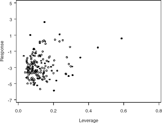
Output 3.1 lists the IDs of the outlying observations (OUTINDI), observed proportion (OBSPROP) and number of observations in the training and test sets (NTRAIN and NTEST) after the first run of Program 3.1. Figure 3.1 contains the plot of the points assigned to each data set.

Example. Output from Second Run of Program 3.1

OUTINDI

                           14        96       140       151       155

                                         OBSPROP

                                           0.712

                                      NTRAIN     NTEST

                                         121        49

Figure 3-2. Final assignment of observations, training set (circle), test set (star) and outlier (dot)

The first run of the program allocated 117 observations (68.8%) to the training set and 53 observations to the test set. The proportion of the observations assigned to the the training set was a bit lower than the desired proportion. Upon visual inspection of the data set definitions, Figure 3.1, it was decided to run the program again only this time allocating 4 observations identified as outliers to the training set (observations 109, 128, 139 and 165). Figure 3.2 contains the plot after the second run of Program 3.1 and the output shows the IDs of the outlying observations, observed proportion and number of observations in each data set after the second run. After the second run, 121 observations (71.2%) were assigned to the training set and 49 observations to the test set.