
14.6. Sequential Designs in Clinical Trials
Sequential design and analysis plays a natural role in clinical trials, primarily because of the ability it gives of stopping early either if the treatment under test does not deliver the anticipated effect, or because it is more efficacious than was thought initially. Most sequential approaches are based on frequentist statistics (see, for example, Armitage (1975) and Whitehead 1997), and normally carried out group sequentially, as data are reviewed and monitored on a periodic basis. There is a long tradition of criticizing such frequentist approaches, firstly because by focussing on the consequences of the stopping rules on the Type I error rate they contradict the likelihood principle (Anscombe, 1963; Cornfield, 1969), and secondly because they ignore the fact that stopping is a decision whose losses should be taken into account.
There are a number of approaches that have been looked at to determine an optimal decision rule in a sequential context. The first is traditionally the way that sequential decisions have been tackled and is based on backward induction (Berger, 1985).
The idea in backward induction is extremely simple and begins by considering the last possible decision that can be made at the point that the final data that could be gathered have been gathered. For every possible data set there is an optimal decision to be made. for example, in the case of the comparison of two treatments: which is the best treatment, or which can be recommended. Associated with the optimal decision is an expected loss in which the expectation is based on the posterior distribution of the parameters. The penultimate decision is considered next. Now there are three potential decisions that could be taken for each possible data set:
Stop and recommend the first treatment.
Stop and recommend the second treatment.
Continue to the final stage.
If the trial is continued, the loss, that includes the cost of the sampling required to reach the final decision point, can be determined, as can the expected losses of each decision to stop. Consequently, the optimal decision and its expected loss can be determined. In principle, the process can be continued backwards in time to the first decision to be made. Such sequential decision problems are famously difficult because
... if one decision leads to another, then to analyse the former, one first needs to analyse the latter, since the outcome of the former depends on the choice of the latter (French, 1989)
A consequence of which is that to completely solve the problem by backward induction involves accounting for exponentially increasing numbers of potential scenarios (Berger, 1985).
The second approach taken to solving sequential decision problems is a forward algorithm based on simulation. Before considering this approach, we will illustrate the idea by using it to determine the optimal sample size as in Section 14.5.
Although the general decision problem formulated in Section 14.3 is seductively simple in its formality, its practical implementation is not always so simple. For complex models the integrations required to determine the optimal Bayes' decision may not be straightforward particularly in multi-parameter, non-linear problems or in sequential decision problems.
Even if the integrations necessary are analytically intractable, the Bayes solution can easily be obtained by simulation. Recall that the Bayesian decision is obtained by minimizing
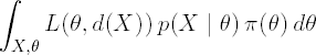
If the loss function L(θ,d(X)) is available for every combination of θ and d(X), the decision problem can be solved as follows. Assuming that the generation of random variables from both π(X|θ) and p(θ) is possible, generate samples {θj,Xj}, j = 1,...,M, and then evaluate for each simulation the loss, L(θj,d(Xj)). An estimate of the expected risk can be obtained from

Numerical optimization of the resulting estimated expected risks gives the optimal Bayesian decision.
In the context of finding optimal sample sizes for a clinical trial discussed in Sections 14.5.1, this approach effectively corresponds to replacing the use of the PROBNORM function by simulation, which is hardly worthwhile. However, the same approach allows the simple relaxation of assumptions. For example, suppose that in Program 14.6 we wish
To use a t-test rather than a test based on a known variance.
To use proper prior information.
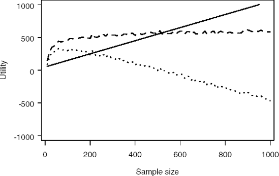
Simulation makes this very simple. Program 14.10 uses simulation to determine the optimal sample size based on a t-statistic when prior information is available both for the treatment effect (using a normal density) and the residual variance (using an inverse-χ2 density). Figure 14.8 plots the computed cost, gain and utility functions.
Example 14-10. Simulating the optimal sample size using t-statistic and informative prior
data nsample;
    n_sim=1000;       /* Number of simulations*/
    alpha=0.05;       /* 2-sided significance level */
    pr_eff_m=35;      /* Prior mean for treatment effect */
    pr_eff_s=100;     /* Prior SD for treatment effect */
    pr_sd=100;        /* Prior expected value of residual SD */
    pr_v=10;          /* Number of df for prior inverse chi-square */
    g=1000;           /* Value of a successful (i.e., significant) trial */
    startc=50;        /* Start-up cost */
    c=1.0;            /* Cost per patient */
    do n=10 to 1000 by 10;
        t_df=n-2; critical=tinv(1-alpha/2,t_df);
        cost=startc+c*n;
        egain=0;
        do i_sim=1 to n_sim;
            theta=pr_eff_m+pr_eff_s*normal(0);
            sigma_2=pr_v*pr_sd**2/(2*rangam(0,pr_v/2));
            y=theta+sqrt(sigma_2*4/n)*normal(0);
            t_statistic=y/(sqrt(sigma_2*4/n));
            if t_statistic>critical then egain=egain+g;
        end;
        egain=egain/n_sim;
        utility=egain-cost;
        output;
    end;
axis1 minor=none label=(angle=90 "Utility") order=(-1000 to 1000 by 500);
axis2 minor=none label=("Sample size") order=(0 to 1000 by 200);
symbol1 i=spline width=3 line=1 color=black;
symbol2 i=spline width=3 line=20 color=black;
symbol3 i=spline width=3 line=34 color=black;
proc gplot data=nsample;
plot (cost egain utility)*n/overlay vaxis=axis1 haxis=axis2 frame;
run;
quit; |
Figure 14-8. Cost (solid curve), expected gain (dashed curve) and utility (dotted curve) as a function of sample size
Of course since we are using simulation techniques we need not be restricted to known, simple, convenient parametric forms for the priors. All that is required is an ability to simulate from the priors.
14.6.1. Sequential Decision Problems
To illustrate how a simulation approach can be used to tackle some sequential decision problems we consider the following example based around the approach taken by Carlin et al (1998). The context is a clinical trial in which the objective is to estimate the treatment effect θ of a new active therapy (A) relative to placebo (P). Large negative values are suggestive of superiority of A over P and conversely large positive values favour P. The protocol allows for a single interim analysis. Along the lines of Freedman and Spiegelhalter (1989) suppose that an indifference region (c2,c1) is pre-determined such that
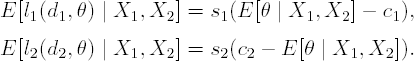
At the final analysis there are two decisions available: d1 to decide in favour of A and d2 to decide in favour of P. For each decision, the loss functions given the true value of θ are:
where s1 and s2 are positive constants. These losses are negatively increasing (gains) for correct decisions. Given the posterior at the final analysis, p(θ | X1, X2), the best decision is determined by the smaller of the posterior expected losses:
By equating these losses and solving for E[θ | X1,X2], it is clear that Decision d1 will be optimal if
otherwise Decision d2 is optimal.
At the interim analysis, in addition to Decisions d1 and d2 to stop in favour of A or P, respectively, based on p(θ | X1), there is a further decision possible, which is to proceed to the final analysis, to incur the extra cost (c3) of the patients recruited between the interim and final analyses and then to make the decision.
If σ2 is known, the forward approach to the decision is algorithmically as follows:
Based on the prior distribution and the first stage data X1, determine the posterior distribution p(θ | X1,σ2).
Determine the expected losses s1(E[θ | X1] − c1) and s2 (c2 − E[θ | X1]).
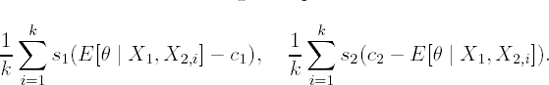
Let k be the number of simulatons. For i = 1 to k,
Simulate θi from p(θ | X1, σ2).
Simulate data X2,i from p(X2 | θi,σ2).
Calculate s1 (E[θ | X1,X2,i] − c1) and s2 (c2 − E[θ | X1,X2,i]).
Let lfinal be the minimum of the following two quantities:
Choose the minimum of

Obvious modifications need to be made if σ2 is unknown.
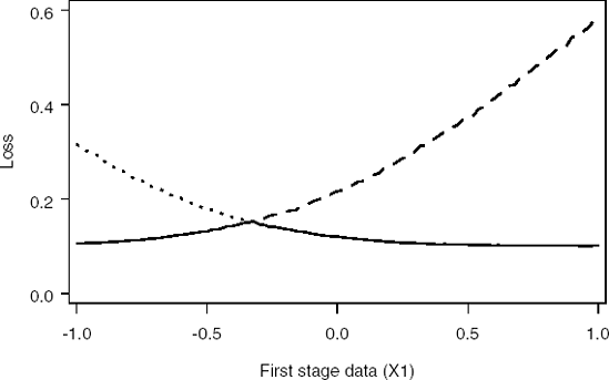
Implementation of this approach is shown in Program 14.11. The output of the program (Figures 14.9 and 14.10) defines regions for the observed treatment difference at the interim for which it is preferable to stop rather than to go on to collect more data and conduct the final analysis.
Example 14-11. Computation of loss functions in the Bayesian sequential design problem
data interim_decision;
    n_sim=10000;   /* Number of simulations*/
    s1=1;          /* Cost associated with falsely choosing d1 (active)*/
    s2=1;          /* Cost associated with falsely choosing d2 (placebo)*/
    s3=0.1;        /* Cost associated with sampling after interim*/
    n1=1;          /* Sample size per group at interim */
    n2=1;          /* Sample size per group after interim */
    sigma_2=0.5**2;/* Known sigma**2 */
    c1=0;          /* Upper indifference boundary (gt favours placebo)*/
    c2=-0.288;     /* Lower indifference boundary (lt favours treatment)*/
    pr_m=0.021;    /* Prior mean */
    pr_sd=0.664;   /* Prior standard deviation */

    /* Looping over an observed treatment effect (n1 patients per group)
 at the interim */
    do x1=-1 to 1 by 0.02;
/* Determine posterior mean (interim) and standard deviation*/
posterior_m_1=(x1*pr_sd**2+2*pr_m*sigma_2/n1)/(pr_sd**2+2*sigma_2/n1) ;
posterior_sd_1=sqrt(1/(1/pr_sd**2+n1/(2*sigma_2)));
/* Determine losses at interim (loss_11: decision 1, loss_21: decision 2) */
loss_11=max(0,s1*(posterior_m_1-c1));
loss_21=max(0,s2*(c2-posterior_m_1));
/* Determine minimum of losses at interim */
loss_interim=min(loss_11,loss_21);
/* Initialise summation variables for future decisions */
loss_12_sum=0; loss_22_sum=0;
/* Simulate future data */
do i_sim=1 to n_sim;
/* Simulate treatment parameter from posterior at interim */
theta=posterior_m_1+posterior_sd_1*normal(0);
/* Simulate treatment effect from n2 patients on each treatment
for given theta */
x2=theta+sqrt(sigma_2*2/n2)*normal(0);
/* Determine posterior mean (final) and standard deviation*/
posterior_m_2=(x2*posterior_sd_1**2+2*posterior_m_1*sigma_2/n2)/
(posterior_sd_1**2+2*sigma_2/n2);
/* Determine losses at final (loss_12: decision 1, loss_22: decision 2) */
loss_12=s3+max(0,s1*(posterior_m_2-c1));
loss_22=s3+max(0,s2*(c2-posterior_m_2));
/* Accumulate losses */
loss_12_sum=loss_12_sum+loss_12;
loss_22_sum=loss_22_sum+loss_22;
end;
/* Calculate expected losses */
loss_12=loss_12_sum/n_sim; loss_22=loss_22_sum/n_sim;
/* Determine minimum of losses at final */
loss_final=min(loss_12,loss_22);
output;
end;
keep loss_11 loss_21 loss_12 loss_22 loss_final loss_interim x1;
axis1 minor=none label=(angle=90 "Loss") order=(0 to 0.6 by 0.2);
axis2 minor=none label=("First stage data (X1)") order=(-1 to 1 by 0.5);
symbol1 i=spline width=3 line=20 color=black;
symbol2 i=spline width=3 line=34 color=black;
symbol3 i=spline width=3 line=1 color=black;
/* Plot loss functions for interim analysis */
proc gplot data=interim_decision;
plot (loss_11 loss_21 loss_interim)*x1/overlay vaxis=axis1 haxis=axis2 frame;
run;
/* Plot loss functions for final analysis */
proc gplot data=interim_decision;
plot (loss_12 loss_22 loss_final)*x1/overlay vaxis=axis1 haxis=axis2 frame;
run;
quit; |
Figure 14-9. Loss functions for Decision 1 (dashed curve), Decision 2 (dotted curve) and minimum loss function (solid curve) at the interim analysis
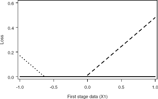
Figure 14-10. Loss functions for Decision 1 (dashed curve), Decision 2 (dotted curve) and minimum loss function (solid curve) at the final analysis
In practice, Carlin et al (1998) use this approach to define a series of critical values for the posterior mean of the treatment effect for each of a number of interims. The advantage of their approach is that the critical values can be determined a priori and there is no need for complex Bayesian simulation during the course of the study. Kadane and Vlachos (2002) develop an alternative approach intended, in their words, to "capitalize on the strengths, and compensate for the weakness of both the backwards and forward strategies."
They develop a hybrid algorithm that works backwards as far as is feasible, determining the expected loss of the appropriate optimal continuation as a "callable function." It then proceeds using the forward algorithm from the trial's start to where the backward algorithm becomes applicable. This reduces the size of the space to be covered and hence will increase efficiency. Berry et al (2000) describe a similar strategy in the context of a dose-response study.