
3.4. Variable Selection
The data used to developed computational models can often be characterized by a few observations and a large number of measured variables, some of which are highly correlated. Traditional approaches to modeling these data are principle component regression (PCR) and partial least squares (PLS) (Frank and Friedman, 1993). The factors obtained from PCR and PLS are usually not interpretable so if the goal is to develop an interpretable model, these are not as useful. By considering the loadings given to each variable, these methods can be used to prune the variables, though the criteria for removing variables can be inconsistent between data sets.
Other popular variable selection procedures are tied to model selection and are often used to when fitting multiple linear regression models, though they can be used with other models, such as a linear discriminant model. A few of the more popular procedures are discussed below. Shrinkage methods are also available to the modeler. Instead of selecting variables, shrinkage methods shrink the regression coefficients by minimizing a penalized error sum of squares, subject to a constraint. In ridge regression, a common shrinkage method, the L2 norm is used as the constraint, and Lasso, another shrinkage method, the L1 norm is used as the constraint.
Best K models examine all possible models and the top K models are selected for further investigation by the modeler. The top models are selected using a measure of fit such as adjusted R2 (R2a) or Mallow's Cp. Since all possible models are examined, the sample size, n, must be strictly greater than the number of descriptors, p. Examining all possible models is computationally intensive and, realistically, this method should be used if p is small. A rule of thumb is p < 11.
Best subset algorithms, such as leaps and bounds (Furnival and Wilson, 1974), do not require the examination of all possible subsets, but use an efficient algorithm to search for the K best models using a statistical criteria such as R2a or Mallow's Cp. It is recommended that other variable selection procedures be used if p > 60.
Stepwise procedures, including forward selection and backward elimination, develop models at each step by adding (forward selection) or deleting (backward elimination) the variable that has the largest (forward selection) or smallest (backward elimination) F-value meeting a particular pre-determined limit. Stepwise procedures are commonly used to build computational models.
The variable selection methods mentioned above are dependent on the type of model being fit and often select variables for the final model which are highly correlated. This is not an issue unless the modeler is interested in an interpretable model. In the following section we present a variable selection method that is based on a stable numerical linear algebra technique. Our technique ranks the predictor variables in terms of importance, taking into account the correlation with the response and the predictor variables previously selected. Our technique deals with the collinearity problem by separating correlated variables during the ranking. Our procedure is a modification of the variable selection procedure proposed by Golub and Van Loan (1996) and is not dependent on the modeler pre-specifying the type of model.
3.4.1. Variable Selection Algorithm
The proposed variable selection algorithm is defined below:
Center the matrix of descriptors, X.
Center the vector of responses, Y.
Calculate Ŷ, where each column is the projection of y onto xi, where x'i is the ith row of X.
Use the Singular-Value Decomposition to calculate the rank of Ŷ.
Apply the QR decomposition with column-pivoting to Ŷ.
The output from the QR decomposition algorithm when column pivoting is invoked is an ordering of the columns of Ŷ. The number of descriptors to use in the model can be obtained from the magnitude of the singular values of the ordered descriptor matrix. This is similar to using a scree plot in PCR to determine the number of directions to use.
The QR decomposition of the matrix X is X = QR, where Q is an orthogonal matrix and R is upper triangular. The matrix Q if formed from the product of p Householder matrices, Hi, i = 1,...,p. A Householder matrix is an elementary reflector matrix. When column-pivoting is incorporated into the QR algorithm, prior to calculating each Householder matrix, the column with the largest norm is moved to the front of the matrix. Since the matrix on which the QR algorithm operates is Ŷ, at each stage the column moved to the front of the matrix will correspond to the descriptor with the highest correlation with y but relatively independent of the previously selected descriptors, xi. In other words, the first column selected will be the descriptor that has the highest correlation with the response. The second column selected will be the descriptor with the highest correlation with the response and the lowest correlation with the first descriptor selected. This continues until all the descriptors have been ordered.
3.4.2. ORDERVARS Module
The variable ordering procedure described in Section 3.4.1 was implemented in a SAS/IML module (ORDERVARS module) that can be found on the book's web site. The inputs to this module are the matrix X of descriptors and the vector y of responses. The outputs are the variable ordering, the rank of X, and a scree plot of the singular values.
The ORDERVARS module starts by centering X and y and then calculates the matrix Ŷ. The QR-algorithm implemented in SAS/IML (QR subroutine) is called.
Column-pivoting is invoked in the QR subroutine by initializing the input vector ORD to all zeros. The ORDERVARS module also creates a SAS data set (SINGVALS) that stores the computed singular values.
3.4.3. Example: Normally Distributed Responses
As an illustrative example, suppose x is distributed N5(0, Σ), where
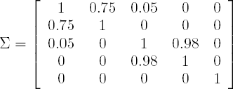
In this example, x1 is correlated with x2 and x3 is highly correlated with x4. Take 25 samples from the above distribution and define
- y = 2x1 + 1.5x3 + x5 + ε,
where ε is distributed N(0,1). The response is a linear function of three of the five descriptors, namely, x1, x3, x5. A variable selection procedure should select 1, 3, 5 as the first three variables.
Program 3.2 provides the code to randomly generate the descriptors for this example and calls the ORDERVARS module on the simulated data. The program starts by initializing the covariance matrix, randomly generating the matrix of descriptors, and then calculating y. To randomly generate data from a multivariate distribution with mean μ and positive-definite covariance matrix Σ, the following transformation was used
- x = Σ1/2z + μ,
where z is a p × 1 vector of observations, zi distributed N(0,1), and the matrix Σ1/2 is the square root matrix of Σ. The square root matrix of a positive definite matrix can be calculated from the spectral decomposition of Σ as:
- Σ1/2 = CD1/2C′,
where C is the matrix of eigenvectors and D is a diagonal matrix whose elements are the square-root of the eigenvalues.
Example 3-2. Variable ordering in the simulated example
proc iml;
    * Initialize Sigma;
    call randseed(564);
    sig={1 0.75 0.05 0 0,
       0.75 1 0 0 0,
       0.05 0 1 0.98 0,
       0 0 0.98 1 0,
       0 0 0 0 1};
    * Calculate sigma^{1/2};
    call eigen(evals,evecs,sig);
    sig12=evecs*diag(evals##0.5)*evecs`;
    * Generate the matrix of descriptors, x;
    n=25;
    x=j(n,5,0);
    do i=1 to n by 1;
    d=j(1,5,.);
    call randgen(d,'normal',0,1);
    x[i,]=(sig12*d`)`;
    end;
    err=j(1,n,.);
    * Randomly generate errors and calculate y;
    call randgen(err,'normal',0,1);
    y=j(n,1,0);
    y=2*x[,1] + 1.5*x[,3] + x[,5] + err`;
    * Concatenate x and y into one matrix;
    xy=x||y;
    * Calculate the correlation matrix;
    cormat=j(6,6,.);
    cormat=corr(xy);
    print cormat[format=5.3];
* Save example data set;
create test from xy[colname={'x1' 'x2' 'x3' 'x4' 'x5' 'y'}];
append from xy;
close test;
use test;
read all var ('x1':'x5') into x;
read all var {y} into y;
* Call the variable selection procedure;
call ordervars(x,y,order,rank);
* Print rank and variable ordering *;
print rank;
print order;
quit; |
Example. Output from Program 3.2
CORMAT

                           1.000 0.808 0.129 0.044 0.175 0.746
                           0.808 1.000 0.014 -.037 0.062 0.511
                           0.129 0.014 1.000 0.977 0.294 0.603
                           0.044 -.037 0.977 1.000 0.308 0.550
                           0.175 0.062 0.294 0.308 1.000 0.576
                           0.746 0.511 0.603 0.550 0.576 1.000

                                           RANK

                                              5

                                          ORDER

1 3 5 2 4 |
After randomly generating the data, the correlation matrix is calculated for the matrix [Xy]. The correlation matrix is given in the Output 3.2. The last row of the correlation matrix corresponds to y. Looking at the correlations, x1 has the highest correlation with the response y and should be selected first by the variable ordering procedure. Output 3.2 also contains the variable ordering produced by the ORDERVARS module. The ordering of the variables is: x1, x3, x5, x2 and x4.
3.4.4. Forward Selection
Let's compare the above results to the results obtained from forward selection. Program 3.3 contains the code to run forward selection in SAS using the REG procedure. The TEST data set used in this program was created in Program 3.2.
Example 3-3. Forward selection on simulated data
proc reg data=test;
    model y = x1 x2 x3 x4 x5/selection=forward;
run; |
Example. Output from Program 3.3
All variables have been entered into the model.

                              Summary of Forward Selection

           Variable     Number     Partial      Model
   Step    Entered      Vars In    R-Square    R-Square     C(p)
      F Value    Pr > F

     1     x1               1       0.5572      0.5572     93.1599
      28.94    <.0001
     2     x4               2       0.2678      0.8250     26.1153
      33.67    <.0001
     3     x5               3       0.0956      0.9206      3.4650
      25.29    <.0001
     4     x2               4       0.0036      0.9242      4.5439
       0.94    0.3432
     5     x3               5       0.0021      0.9263      6.0000
0.54 0.4698 |
Output 3.3 contains the output from Program 3.3. Using forward selection, the variables are entered x1, x4, x5, x2, x3, which is different from the variables used to generate y.
3.4.5. Variable Ordering in the Solubility Data
Program 3.4 executes the ORDERVARS module on the solubility training set. The solubility training and test sets (SOLTRAIN and SOLTEST data sets) were generated in Program 3.1. At the end of Program 3.4 the training and test data sets are created using the new variable ordering and they are stored as SAS data sets (SOLTRUSE and SOLTSUSE data sets).
Example 3-4. Variable ordering in the solubility data
proc iml;
    use soltrain;
    read all var ('x1':'x21') into x;
    read all var {y} into y;
    * Call the variable ordering module;
    call ordervars(x,y,order,rank);
    print rank;
    print order;
    * Store the variable ordering;
    create solorder var{order};
    append;
    close solorder;
    * Create the training and test sets using the new variable order;
    * Store the training and test sets;
    trxy=x[,order[1,]]||y;
    create soltruse from trxy[colname=('x1':'x21'||'y')];
    append from trxy;
    close soltruse;
    use soltest;
    read all var ('x1':'x21') into tsx;
    read all var {y} into tsy;
    tsxy=tsx[,order[1,]]||tsy;
    create soltsuse from tsxy[colname=('x1':'x21'||'y')];
    append from tsxy;
    close soltsuse;
    * Number of observations in the train and test data set;
    ntrain=nrow(trxy); ntest=nrow(tsxy);
    print ntrain ntest;
    quit;
* Vertical axis;
axis1 minor=none label=(angle=90 "Singular value") order=(0 to 12000 by 2000) width=1;
* Horizontal axis;
axis2 minor=none label=("Index") order=(1 to 21 by 1) width=1;
symbol1 i=none value=dot color=black height=5;
proc gplot data=singvals;
plot singularvalues*index/vaxis=axis1 haxis=axis2 frame;
run;
quit; |
Figure 3-3. Singular values in the solubility data set

Example. Output from Program 3.4
RANK

                                              21

                                          ORDER
                  COL1      COL2      COL3      COL4      COL5      COL6      COL7

        ROW1         8        13         3         1        21         9        19

                                          ORDER
                  COL8      COL9     COL10     COL11     COL12     COL13     COL14

        ROW1        12        20         2         4         5        16        10

                                          ORDER
                 COL15     COL16     COL17     COL18     COL19     COL20     COL21

        ROW1         6        17        18         7        14        15        11

                                      NTRAIN     NTEST

121 49 |
Figure 3.3 is a plot of the singular values for each descriptor. Based on this plot it appears only five descriptors are needed to build a predictive model, but sequential regression should probably be used to determine the number of descriptors needed in the model. In sequential regression the variables can be added in order, provided that a certain statistical criterion is met. An example is provided in Section 3.5.1. Output 3.4 contains the variable ordering (ORDER) as well as the number of observations in the training and test data sets (NTRAIN and NTEST).