
14.5. Optimal Sample Size
The Phase III investment example resembles investment problems from other industries, e.g., oil drilling examples described in Raiffa and Schlaifer (1961, Section 1.4.3). One important difference is that Phase III development consists of experiments which we are to design and whose results can be modelled with standard statistical methods. The power, or probability of showing superiority, in one clinical trial is easily determined given the response distributions and test method. The response distributions are typically determined by parameters such as mean effect and standard deviation. Furthermore, these parameters can be modelled using previous clinical (and sometimes preclinical) data (Pallay and Berry, 1999; Burman et al, 2005).
So far, in Sections 14.2 and 14.4, we have taken the Phase III programme to be fixed (if it is run at all). The design of these trials is, however, of utmost importance and definitely a field where statisticians have a lot to contribute. In this section we will consider one single design feature: the trial's sample size.
Decision analytic approaches to sample size calculations in clinical trials have been considered in a variety of situations. General Bayesian approaches are outlined by Raiffa and Schlaifer (1961, Section 5.6) and Lindley (1997). Claxton and Posnett (1996) as well as O'Hagan and Stevens (2001) apply such ideas to clinical trials with health economics objectives. Gittins and Pezeshk (2000) and Pallay (2000) discuss the sizing of Phase III trials, considering regulatory requirements. A review of Bayesian approaches to clinical trial sizing is provided by Pezeshk (2003).
Sample size has often been viewed as a relatively simple function of the following parameters:
"Least clinically relevant effect" δ.
Standard deviation σ.
Power 1 − β.
One-sided significance level α/2.
In a two-arm trial of reasonable size, so that a normal approximation is appropriate, the total sample size is given by

where Φ(·) is the standard normal cumulative distribution function.
The main difficulty in sample size calculations is the choice of α, β, δ and σ. The one-sided significance level α is conventionally set at a 2.5% level so that the two-sided size of the test is 5% (FDA, 1998). The standard deviation σ is sometimes hard to estimate at the planning stage and a misspecification may distort the resulting sample size considerably. However, there is often enough data from previous smaller trials with the test drug and from Phase III trials of other drugs with the same response variable for a reasonably robust guess of the value of σ.
More interesting parameters are β and, even more so, the treatment effect δ. We will start by looking at the optimal power when δ is naïvely taken as a fixed known value. After that we will discuss δ.
The power, 1 − β, is often conventionally set at 90%. This is indeed convenient for the statistician performing the sample size calculation as he or she does not have to consider the context around the trial. The importance of the trial, cost of experimentation, recruitment time and other factors are simply ignored. We argue, however, that the choice of the sample size is often a critical business decision. A Phase III programme or even a single mortality trial will often cost in the order of 100 MUSD (DiMasi et al, 2003). Changing the power from 80% to 90%, or from 90% to 95%, can result in a considerable increase of the trial's cost, sometimes tens of MUSD. In addition, and often even more importantly, the time to marketing may be delayed. For such important decisions, a decision analysis framework seems natural.
14.5.1. Optimal Sample Size Given a Fixed Effect
We will start with a very simple decision analysis model and then gradually add some features that can increase the realism of the model. Suppose that a statistically significant trial result in favour of the test drug will lead to regulatory approval and a subsequent monetary gain G for the company. Think of G as the expected discounted net profit during the whole product life-cycle, where sale costs (production, distribution, promotion, etc) are subtracted from the sales. In the case of a non-significant result, the drug will not be approved and there will be no gain.
Assume that the cost for conducting a clinical trial with N > 0 patients is C(N) = C0 + cN, where C0 is the start-up cost and c is the cost per patient. If no trial is conducted, we have N = 0 and C(0)=0. The trial cost and other development costs should not be included in G. The company profit is assumed to be GI{S} − C(N), where I{S} = 1 if the trial is statistically significant and 0 otherwise. Note that this assumption is typically not realistic, as the magnitude of the estimated effect as well as the precision of the estimate are likely to affect the sales. Furthermore, the times of submission, approval and marketing are likely to depend on N. The model can be made more realistic by incorporating such aspects, this is partly done in Section 14.5.3 below.
Under these assumptions, the expected profit is given by
where p(N) is the probability of a significant outcome, i.e., power. The values of the parameters vary considerably depending on the drug and therapeutic area. For the sake of illustration, assume that the effect size δ/σ = 0.2, value of the trial G = 1000, start-up cost C0 = 50 and cost per patient c = 0.1. Program 14.6 computes the profit function for the selected parameter values.
Example 14-6. Computation of costs and gains in a Phase III trial
data npower;
    alpha=0.05;    /* Two-sided significance level */
    critical=probit(1−alpha/2);
    effsize=0.2;   /* Effect size */
    g=1000;        /* Value of successful (i.e., significant) trial */
    startc=50;     /* Start-up cost */
    c=0.1;         /* Cost per patient */
    do n=0 to 2000 by 10;
        power=probnorm(effsize*sqrt(n/4)-critical);
        egain=g*power;
        cost=startc+c*n;
        profit=egain-cost;
        output;
    end;
run;
axis1 minor=none label=(angle=90 "Utility") order=(0 to 1000 by 200);
axis2 minor=none label=("Sample size") order=(0 to 2000 by 500);
symbol1 i=join width=3 line=1 color=black;
symbol2 i=join width=3 line=20 color=black;
symbol3 i=join width=3 line=34 color=black;
proc gplot data=npower;
    plot (cost egain profit)*n/overlay nolegend haxis=axis2 vaxis=axis1;
    run;
quit; |
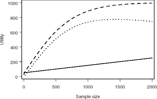
Figure 14.4, generated by Program 14.6, depicts the resulting profit function. The maximum profit is achieved at N = 1431 patients. This corresponds to the probability of a significant outcome (power) of 96.6%.
Figure 14-4. Cost (solid curve), expected gain (dashed curve) and expected profit (dotted curve) as a function of sample size
It is clear that Program 14.6 relies on a fairly inefficient algorithm. It simply loops through all values of N between 0 and 2000 to find the sample size that maximizes the expected net gain. A more efficient approach is to explicitly formulate this problem as an optimisation problem and utilise one of many optimization routines available in SAS. In principle, it would have been possible to use a decision tree (i.e., PROC DTREE) for this optimization problem. However, since so many different values of N are possible, it is more convenient to treat it as an approximately continuous variable and use the optimization procedure PROC NLP.
The NOPT macro in Program 14.7 calculates the optimal sample size using the NLP procedure. The procedure maximizes the value of PROFIT (expected net gain) with respect to the N variable (total sample size). The underlying assumptions are identical to the assumptions made in Program 14.6, i.e., the effect size δ/σ = 0.2, value of the trial G = 1000, start-up cost C0 = 50 and cost per patient c = 0.1.
Example 14-7. Optimal sample size
%macro nopt(effsize,g,startc,c,alpha);
    proc nlp;
        ods select ParameterEstimates;
        max profit; /* Maximise the expected net gain */
        decvar n;      /* Total sample size */
        critical=probit(1-&alpha/2);
        power=probnorm(&effsize*sqrt(n/4)-critical);
        egain=&g*power;
        cost=&startc+&c*n;
        profit=egain-cost;
    run;
%mend nopt;
%nopt(effsize=0.2,g=1000,startc=50,c=0.1,alpha=0.05); |
Example. Output from Program 14.7
PROC NLP: Nonlinear Maximization

                                      Optimization Results
                                       Parameter Estimates
                                                               Gradient
                                                              Objective
                           N Parameter         Estimate        Function

1 n 1431.412256 1.336471E-9 |
Output 14.7 shows that the optimal sample size is 1431 patients. This value is identical to the optimal sample size computed in Program 14.6. Some robustness checks are easily implemented by varying the assumed effect size. For example, it is easy to verify that the optimal sample sizes for δ/σ = 0.15 and δ/σ = 0.25 are N = 2164 and N = 1018 patients, respectively.
The model used hitherto in this subsection is generally too simplistic to be of practical value. We will return to the uncertainty in treatment effect in Section 14.5.3 but first, in the next subsection, comment on the number of significant trials needed for regulatory approval.
14.5.2. The Optimal Number of Trials
Often two statistically significant trials are needed for regulatory approval. Assume that two virtually identical trials, each of size N should be run and that both are required to be significant.
The reasoning used in Section 14.5.1 can then easily be extended to give
which can be optimised using a slightly modified version of Program 14.6.
Provided that the two trials have equal conditions, it is optimal to have the same sample size in both trials. Often the trials are, however, conducted in different countries and in different populations. Costs, recruitment times and anticipated effects may therefore vary and non-equal sample sizes may be indicated.
The probability of achieving significant results in at least two trials is typically higher if a fixed number of patients is divided into three trials instead of two. In fact, it is easier to get significances in two trials and supportive results in the third (defined as a point estimate in favour of the new drug) when three trials are run than to get significances in both trials when two trials are run. One numerical illustration is provided by Program 14.8. Success of the trial program is defined as all trials giving positive point estimates and at least two trials being statistically significant at the conventional level.
Example 14-8. Optimal number of trials
data no_of_trials;
    alpha=0.05;
    effect=20;
    sd=100;
    n_tot=2000;
    critical=probit(1-alpha/2);
    format m n 5.0 p_sign p_supp p_success 5.3;
    do m=1 to 5;
        n=n_tot/m;
        p_sign=probnorm(effect/sd*sqrt(n/4)-critical);
        p_supp=probnorm(effect/sd*sqrt(n/4));
        p_cond=p_sign/p_supp;
        p_success=p_no_neg*(1-probbnml(p_cond,m,1));
        output;
    end;
    label m='Number of trials'
          n='Sample size'
          p_sign='Prob of significance'
          p_supp='Prob of supportive results'
          p_success='Success probability';
    keep m n p_sign p_supp p_success;
proc print data=no_of_trials noobs label;
run; |
Example. Output from Program 14.8
Number                               Prob of
                    of      Sample      Prob of       supportive      Success
                  trials     size     significance     results      probability

                      1      2000        0.994          1.000          0.000
                      2      1000        0.885          0.999          0.784
                      3       667        0.733          0.995          0.816
                      4       500        0.609          0.987          0.798
5 400 0.516 0.977 0.754 |
Output 14.8 lists several variables, including success probability when a total sample size is divided equally in m trials (m = 1,...,5). With a single trial, the probability of regulatory success is zero, as two significant trials are needed. Interestingly, the success probability increases when going from two to three trials.
From a regulatory perspective, it is probably undesirable that sponsors divide a fixed sample size into more than two trials without any other reason than optimisation of the probability for approval. The regulators should therefore apply such rules that do not promote this behaviour. This is a simple example of the interaction between different stakeholders' decision analyses.
In fact, the reason that regulators require two trials to be significant is not entirely clear. Say that two trials are run and each is required to be significant at a one-sided 0.025 level (i.e., α = 1/40) and registration follows only when both trials are significant. This corresponds to an overall Type I error rate of (1/40)2 = 1/1600 = 0.000625. However if centres, patients and protocols are regarded as exchangeable between the two trials, then an equivalent protection in terms of Type I error rate can be provided to the regulator using fewer patients for equivalent overall power (Senn, 1997; Fisher, 1999; Rosenkranz, 2002; Darken and Ho, 2004). In fact, one could run two such trials and simply pool their results together for analysis. The difference between the resulting pooled trial rule and the conventional two-trials rule in terms of the critical values of the standard normal distribution is illustrated in the accompanying Figure 14.5 taken from Senn (1997).
In this figure, the boundaries for significance are plotted in the {Z1,Z2} space, where Z1 is the standardised test statistic for the first trial and Z2 for the second. For the two trials rule we require that both Z1 > 1.96 and {Z2 > 1.96}. The resulting critical region is that above and to the right of the dashed lines. For the pooled trial rule we require (Z1 + Z2)/√2 > 3.227. The latter rule may be derived by noting that Var(Z1 + Z2) = 2 and 1 − Φ(3.227) ≈ 0.000625. The associated critical region is above and to the right of the solid line.
Figure 14-5. Rejection regions for the pooled-trial and two-trial rules

If we calculate power functions for the pooled- and two-trial rules as a function of the standardised non-centrality parameter, δ* for a single trial, then this has the value 2δ*/√2 = √2δ* for the pooled-trial rule. Bearing in mind that both trials must be significant for the two-trial rule, the power functions are
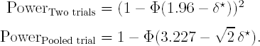
Figure 14.6 displays a plot of the two power functions. It can be seen from the figure that the power of the pooled-trial rule is always superior to that of the two trial rule.
Figure 14-6. Power of the pooled-trial (solid curve) and two-trial (dashed curve) rules

One argument for preferring two trials to such a single trial would be if the trials were not exchangeable and had different design details either in terms of type of centre and patient or in terms of protocol. Two trials that were both significant at a 0.025 level would then be more impressive in terms of robustness than a single trial significant at a 0.000625 level. There is, however, no evidence that in their Phase III programmes clinical trial sponsors deliberately choose trials that differ in design nor that regulators require them to. For regulatory thinking on this issue, see Committee for Proprietary Medicinal Products (CPMP) (2001).
14.5.3. A Bayesian Approach to Sample Size Calculations
We have, in Section 14.5.1, looked at the optimal sample size given a fixed treatment effect δ. However, the main problem in deciding on whether to conduct the trial at all and, in that case, how to choose a sample size lies in the uncertainty regarding this parameter. If δ could be objectively established with good precision at this stage, there would be little need to conduct a clinical trial in order to estimate it. Hence, clearly we cannot insert the true value of δ in the power formula, if we regard this as being the effect of the treatment. It may also be misleading to insert a point estimate based on previous data, due to the uncertainty of this estimate. It is often recommended that the sample size calculation should be based on the "least clinically significant effect" but even this is a quantity that cannot be established with absolute precision, since physicians may disagree between themselves and even from time to time, as to what it is.
To decide on whether to invest in a Phase III programme a clinical trial sponsor must clearly have some sort of prior opinion about either the size of the effect that would be important or the size that would be likely to obtain. We think that it is reasonable to try to formalise this opinion using a Bayesian prior distribution. However, we warn here that the solution we describe below is not fully Bayesian and may be far from optimal because it does not model utility explicitely as a function of the treatment effect.
Fully Bayesian sample size determinations (with or without utility) have been discussed by several authors, e.g., Lindley (1997) and Pezeshk (2003). We will, however, investigate an approach where Bayesian decision theory is used only for in-house company decisions, such as designing the clinical program, see, for example, Gittins and Pezeshk (2000). Solely frequentist analyses of clinical trial results are communicated externally to regulators and the public. This dichotomy between internal Bayesianism and external frequentism is motivated by the stakeholder situation. The sponsor conducts the trial program in order to provide information to regulators and prescribing physicians on which they can base their decisions. These stakeholders will base their decisions on the data, for convenience often presented as frequentist confidence intervals, and possibly on their own priors. For the sponsor, the optimal program design depends on its own prior and on the anticipated reaction of other stakeholders. The questions to investigate are of the type: What is the probability that the proposed design will lead to trial results that will convince regulators to approve the marketing of our drug and convince physicians to prescribe the drug?
Program 14.9 calculates expected utilities by integrating over the prior distribution for the treatment effect δ (integration is performed using the QUAD function of SAS/IML). This prior distribution is assumed to be normal and its mean and standard deviation are given by the MUE and MUSE variables, respectively (notice that the case when MUSE = 0 corresponds to a model with a known treatment effect). SD is the residual standard deviation. The value of MUE, SD and some other parameters of the program are chosen to facilitate the comparison with the approach described in Section 14.5.1. For example, the effect size is centered around 0.2, the start-up cost is 50 and cost per patient is 0.1.
The program also allows for a possible non-inferior (but non-superior) result. If this option is not applicable, let NIMARGIN=0. The maximal possible value following a non-inferior result is given by the parameter VNIMAX and, similariliy, VSUPMAX is the maximal value of a superior result.
In addition to the options of including a prior effect distribution and/or a non-inferiority criterion, a time delay due to increased sample size may also be included. In the model, the maximal profit given marketing (VNIMAX or VSUPMAX) is decreased by a factor TIMEC times the sample size.
In the DO loop in Program 14.9, the expexted utility (EUTILITY) is calculated for a number of different sample sizes (given by the vector SIZE). On the negative side, TOT_COST is the total cost for the trial and TIME_FACTOR accounts for the relative loss in value due to the time delay. PSUP and PNI are the probabilities for superiority and non-inferiority, respectively. These are functions of the treatment EFFECT. Given the EFFECT, UTILITY is the expected gain, that is, probability-weighted profit corrected for the time delay via TIME_FACTOR, minus the total cost of running the trial. QUAD is applied to calculate the expected utility over the prior distribution for the effect.
In the model underlying the program, the trial result is only important for the regulatory label (superior, non-inferior, or not approved). Given the label, the profit in this model is independent of the trial result and sample size. If one is trying to apply decision analysis on a practical Phase III sizing problem, we advise that the modeling of the profit is done with greater care. If a better commercial model can be defined in terms of sample size and trial results, it is often relatively straightforward to modify Program 14.9 accordingly.
Example 14-9. Expected utility when the treatment effect is uncertain
proc iml;
    muE=20;
    muSE=10;
    sd=100;
    NImargin=10;
    vSUPmax=1000;
    vNImax=400;
    alpha=0.05;
    crit=probit(1−alpha/2);
    timec=0.0001;
    startc=50;
    c=0.1;
size=t(do(0,2000,10));
m=nrow(size);
Eutility=j(m,1,0);
do k=1 to m;
n=size[k,1];
time_factor=max(1-timec*n,0);
tot_cost=startc+n*c;
start h(effect) global(n,muE,muSE,sd,NImargin,crit,
vSUPmax,vNImax,time_factor,tot_cost);
pSup=probnorm(effect/sd*sqrt(n/4)-crit);
pNI=probnorm((effect+NImargin)/sd*sqrt(n/4)-crit)-pSup;
utility=time_factor*(vSUPmax*pSup+vNImax*pNI)-tot_cost;
density=exp(-(effect-muE)**2/(2*muSE**2))/sqrt(2*3.14159*muSE**2);
h_out=density*utility;
return(h_out);
finish;
call quad(temp,"h",{.M .P}); /* Integrate over the real axis */
Eutility[k,1]=temp;
end;
create plotdata var{size Eutility};
append;
quit;
axis1 minor=none label=(angle=90 "Utility") order=(0 to 600 by 200);
axis2 minor=none label=("Sample size") order=(0 to 2000 by 500);
symbol1 i=join width=3 line=1 color=black;
proc gplot data=plotdata;
plot Eutility*size/haxis=axis2 vaxis=axis1 frame;
run;
quit; |
Figure 14-7. Expected utility as a function of sample size

The output of Program 14.9 is displayed in Figure 14.7. The figure depicts the relationship between the expected utility and total sample size. Under the assumptions made in the program, the optimal sample size is 887 patients, which is much smaller than the optimal sample size of 1431 patients for the model considered in Section 14.5.1.
14.5.4. Do Not Sub-Optimise!
A poor decision analysis, which ignores essential components of the problem, is often worse than no formal decision analysis at all. As Einstein said, "Things should be made as simple as possible—but no simpler". We would therefore like to stress that the models presented in Sections 14.5.1 and 14.5.3 must not be applied thoughtlessly to a practical problem. They should be seen just as examples of how a decision model can be built and refined and how to analyze continuous decision problems using SAS. Additional factors which may be important in a practical situation are the demand for safety data, the relation between the amount of Phase III data and sales, alternative investment options in terms of other drugs in the pipeline, etc.
14.5.5. Integrating the Models
Many problems involve a number of decisions, which have to be taken at different times. Earlier decisions may lead to information that can be used as input for later decisions. This is obvious in clinical development where the final decisions concerning the design of the Phase III trials will be taken after the analysis of a dose-finding trial (Phase IIb), which might follow upon a proof of principle trial (Phase IIa) and so forth. Such problems, involving sequential decisions, are often best attacked by backward induction (Bather, 2000); the analysis starts by solving the decision problems at the latest stage and then works gradually backwards in time to reach an optimal solution of the entire sequential problem.
The drug development decision model of Sections 14.2 and 14.4, focussing on go/no go decisions, is naturally connected with the sample size decisions studied in the present section. Consider for a moment the integrated decision problem with the three questions:
Should a pretest be run?
Should a Phase III trial be run?
What is the optimal sample size in a Phase III trial?
The best way to solve the composite problem is by starting to analyse the latest decision. The optimal sample size is determined for all the different scenarios, e.g.,
Scenario 1: A positive pretest,
Scenario 2: A negative pretest,
Scenario 3: No pretest to be run,
and the corresponding conditional expected utility is calculated. Then, these values can be used as rewards in a decision tree that contains only the pretest and Phase III go/no go decisions. Similarly, PROC DTREE is working by backward induction and analyses the latest nodes first, taking expectation over chance nodes and maximizing over decision nodes.
Yin (2002) analyses sample sizing in Phase II trials in light of a future go/no go decision.