
12.7. MNAR Modeling
Even though the assumption of likelihood ignorability encompasses the MAR and not only the more stringent and often implausible MCAR mechanisms, it is difficult to exclude the option of a more general MNAR mechanism. One solution for continuous outcomes is to fit an MNAR model as proposed by Diggle and Kenward (1994). In the discrete case, Molenberghs, Kenward, and Lesaffre (1997) considered a global odds ratio (Dale) model.
However, as pointed out in the introduction and by several authors (discussion to Diggle and Kenward, 1994; Verbeke and Molenberghs 2000, Chapter 18), we must be extremely careful with interpreting evidence for or against MNAR in a selection model context, especially in large studies with a lot of power. We will return to these issues in Section 12.8.
12.7.1. Diggle-Kenward Model
To be consistent with notation introduced in Section 12.3, we assume a vector of outcomes Yi is designed to be measured. If dropout occurs, Yi is only partially observed. We denote the occasion at which dropout occurs by Di > 1, and Yi is split into the (Di – 1)-dimensional observed component Yio and the (ni – Di + 1)-dimensional missing component Yimi. In case of no dropout, we let Di = ni + 1, and Yi equals Yio. The likelihood contribution of the ith subject, based on the observed data (yio, di), is proportional to the marginal density function
in which a marginal model for Yi is combined with a model for the dropout process, conditional on the response, and where θ and ψ are vectors of unknown parameters in the measurement model and dropout model, respectively.
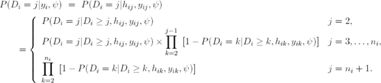
Let hij = (yi1,...,yi;j-1) denote the observed history of subject i up to time ti,j-1. The Diggle-Kenward model for the dropout process allows the conditional probability for dropout at occasion j, given that the subject was still observed at the previous occasion, to depend on the history hij and the possibly unobserved current outcome yij, but not on future outcomes yik, k > j. These conditional probabilities P(Di = j|Di ≥ j, hij, yij, ψ) can now be used to calculate the probability of dropout at each occasion:
Diggle and Kenward (1994) combine a multivariate normal model for the measurement process with a logistic regression model for the dropout process. More specifically, the measurement model assumes that the vector Yi of repeated measurements for the ith subject satisfies the linear regression model Yi ∼ N(Xi β, Vi), i = 1, ..., N. The matrix Vi can be left unstructured or assumed to be of a specific form, e.g., resulting from a linear mixed model, a factor-analytic structure, or spatial covariance structure (Verbeke and Molenberghs, 2000).
In the particular case that a linear mixed model is assumed, one writes (Verbeke and Molenberghs, 2000)
where Yi is the n dimensional response vector for subject i, 1 ≤ i ≤ N, N is the number of subjects, Xi and Zi are (n × p) and (n × q) known design matrices, β is the p dimensional vector containing the fixed effects, bi ~ N(0, G) is the q dimensional vector containing the random effects. The residual components εi ~ N(0, Σi).
The logistic dropout model can, for example, take the form
More general models can easily be constructed by including the complete history hij = (yi1,...,yi;j-1), as well as external covariates, in the above conditional dropout model. Note also that, strictly speaking, we could allow dropout at a specific occasion to be related to all future responses as well. However, this is rather counter-intuitive in many cases. Moreover, including future outcomes seriously complicates the calculations since computation of the likelihood (12.7.14) then requires evaluation of a possibly high-dimensional integral. Note also that special cases of model (12.7.16) are obtained from setting ψ2 = 0 or ψ1 = ψ2 = 0, respectively. In the first case, dropout is no longer allowed to depend on the current measurement, implying MAR. In the second case, dropout is independent of the outcome, which corresponds to MCAR.
Diggle and Kenward (1994) obtained parameter and precision estimates by maximum likelihood. The likelihood involves marginalization over the unobserved outcomes Yim. Practically, this involves relatively tedious and computationally demanding forms of numerical integration. This, combined with likelihood surfaces tending to be rather flat, makes the model difficult to use. These issues are related to the problems to be discussed next.
Apart from the technical difficulties encountered during parameter estimation, there are further important issues surrounding MNAR based models. Even when the measurement model (e.g., the multivariate normal model) would beyond any doubt be the choice of preference for describing the measurement process should the data be complete, then the analysis of the actually observed, incomplete version is, in addition, subject to further untestable modeling assumptions.
When missingness is MAR, the problems are less complex, since it has been shown that, in a likelihood or Bayesian framework, it is sufficient to analyze the observed data, without explicitly modeling the dropout process (Rubin 1976, Molenberghs and Verbeke 2000). However, the very assumption of MAR is itself untestable. Therefore, ignoring MNAR models is as little an option as blindly shifting to one particular MNAR model. A sensible compromise between considering a single MNAR model on the one hand or excluding such models from consideration on the other hand, is to study the nature of such sensitivities and, building on this knowledge, formulate ways for conducting sensitivity analyses. Indeed, a strong conclusion, arising from most sensitivity analysis work, is that MNAR models have to be approached cautiously. This was made clear by several discussants to the original paper by Diggle and Kenward (1994), in particular by Laird, Little, and Rubin. An implication is that, for example, formal tests for the null hypothesis of MAR versus the alternative of MNAR, should be approached with the utmost caution, a topic studied in detail by Jansen et al (2005). These topics are taken up further in Section 12.8.
12.7.2. Implementation of Selection Models in SAS
We have developed a series of SAS programs to implement a special case of the Diggle-Kenward approach. For the measurement process, we considered a more specific case of model (12.7.15), with various fixed effects, a random intercept, and allowing Gaussian serial correlation. This means the covariance matrix Vi becomes
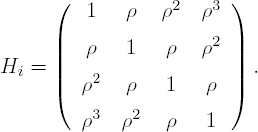
where Jn is an n × n matrix with all its elements equal to 1, In is the n × n identity matrix, and Hi is determined through the autocorrelation function ρujk, with ujk the Euclidean distance between tij and tik, i.e.,

The proposed SAS implementation can easily be adapted for another form of model (12.7.15), by just changing this Vi matrix.
Program 12.7, available on the book's companion Web site, plays the central role in fitting the Diggle-Kenward model. The following arguments need to be provided to the program:
X and Z matrices that contain all Xi and Zi design matrices (i = 1,...,N).
Y vector of all Yi response vectors (i = 1,...,N).
INITIAL is a vector of initial values for the parameters in the model.
NSUB and NTIME are the number of subjects N and the number of time points n respectively.
Within Program 12.7, the INTEGR module calculates the integral over the missing data and the LOGLIK module evaluates the log-likelihood function L(θ, ψ). Finally, the log-likelihood function is maximized. Diggle and Kenward (1994) used the simplex algorithm (Nelder and Mead, 1965) for this purpose and Program 12.7 relies on the Newton-Raphson ridge optimization method (NLPNRR module of SAS/ILM) since it combines stability and speed. However, in other analyses, it may be necessary to try several other optimization methods available in SAS/IML.
The following NLPNRR call is used in the program:
call nlpnrr(rc,xr,"loglik",initial,opt,con);
Here, LOGLIK is the module of the function we want to maximize. The initial values to start the optimization method are included in the INITIAL vector. The OPT argument indicates an options vector that specifies details of the optimization process: OPT[1]=1 request maximization and the amount of output is controlled by OPT[2]. A constraint matrix is specified in CON, defining lower and upper bounds for the parameters in the first two rows (d>0, r2>0 and σ2>0). Finally, all optimization methods return the following results: the scalar return code, RC, and a row vector, XR. The return code indicates the reason for the termination of the optimization process. A positive return code indicates successful termination, whereas a negative one indicates unsuccessful termination. That is, that the result in the XR vector is unreliable. The XR vector contains the optimal point when the return code is positive.
Next, the program also calls the NLPFDD module, which is a subroutine that approximates derivatives by finite differences method,
call nlpfdd(maxlik,grad,hessian,"loglik",est);
Here, again LOGLIK is the module of the log-likelihood function. The vector that defines the point at which the functions and derivatives should be computed is EST. This module computes the function values MAXLIK (which is in this case the maximum likelihood, since EST is the maximum likelihood estimate) the gradient vector GRAD, and the Hessian matrix HESSIAN, which is needed to calculate the information matrix, and thus the standard errors STDE.
12.7.2.1. Analysis of Exercise Study Data
The program for fitting the Diggle-Kenward model is now applied to the analysis of the exercise study data. We will fit the model under the three different missingness mechanisms, MCAR, MAR and MNAR. Further, we will also expand the logistic regression for the dropout model by allowing it to depend on covariates.
To obtain initial values for the parameters of the measurement model, Program 12.5 fits a linear mixed model to the exercise data using PROC MIXED. We assume a linear trend within each treatment group, which implies that each profile can be described with two parameters (intercept and slope). The error matrix is chosen to be of the form (12.7.17). For subject i = 1,...,50 on time point j = 1,...,4, the model can be expressed as
- Yij = β0 + β1 (groupi − 1) + β2 tj (groupi − 1) + β3 tj groupi + εij,
where εi ~ N(0, Vi) and Vi = dJ4 + σ2I4 + τ2Hi, with
The intercept for the placebo group is β0 + β1, and the intercept for the treatment group is β0. The slopes are β2 and β3, respectively.
Example 12-5. Linear mixed model in the exercise study example
proc mixed data=exercise method=ml;
    class group id;
    model y=group time*group/s;
    repeated/type=ar(1) local subject=id;
    random intercept/type=un subject=id;
run; |
The parameter estimates from the fitted linear mixed model (Program 12.5) are shown in Table 12.5 and will later be used as initial values in Program 12.7.
| Parameter | Estimate | Initial value |
|---|---|---|
| β0 | −0.8233 | −0.82 |
| β1 | 0.1605 | 0.16 |
| β2 | 0.9227 | 0.92 |
| β3 | 1.6451 | 1.65 |
| d | 2.0811 | 2.08 |
| τ2 | 0.7912 | 0.79 |
| ρ | 0.4639 | 0.46 |
| σ2 | 0.2311 | 0.23 |
Further, initial values for the parameters of the dropout model are also needed. As mentioned before, we will fit three models in turn, under the MCAR (ψ1 = ψ2 = 0), MAR (ψ2 = 0) and MNAR mechanisms, respectively. The initial values for these parameters are given in Table 12.6.
| Dropout Mechanism | ||||
|---|---|---|---|---|
| Parameter | MCAR | MAR | MNAR | MNAR + Covariate |
| ψ0 | 1 | |||
| ψ1 | 1 | |||
| ψ2 | 1 | |||
| γ | 1 | |||
The parameters that will later be passed to Program 12.7 (X and Z matrices, Y and INITIAL vectors and NSUB and NTIME parameters) are created using PROC IML. Program 12.6 illustrates the process of creating these variables when the missingness mechanism is MCAR.
Example 12-6. Creating matrices, vectors and numbers necessary for Program 12.7
proc iml;
    use exercise;
    read all var {id group time y} into data;
    id=data[,1];
    group1=data[,2];
    group0=j(nrow(data),1,1)-group1;
    time=data[,3];
    timegroup0=time#group0;
    timegroup1=time#group1;
intercept=j(nrow(data),1,1);
create x var {intercept group0 timegroup0 timegroup1}; append;
y=data[,4];
create y var {y}; append;
z=j(nrow(y),1,1);
create z var {z}; append;
beta=-0.82//0.16//0.92//1.65;
D=2.08;
tau2=0.79;
rho=0.46;
sigma2=0.23;
psi=1;
initial=beta//D//tau2//rho//sigma2//psi;
create initial var {initial}; append;
nsub=50;
create nsub var {nsub}; append;
ntime=4;
create ntime var {ntime}; append;
quit; |
Program 12.7 fits the Diggle-Kenward model under the MCAR assumption. To save space, the complete SAS code is provided on the book's companion Web site.
Example 12-7. Diggle-Kenward model under the MCAR assumption in the exercise study example
proc iml;
    use x; read all into x;
    use y; read all into y;
    use z; read all into z;
    use nsub; read all into nsub;
    use ntime; read all into ntime;
    use initial; read all into initial;
    g=j(nsub,1,0);
    start integr(yd) global(psi,ecurr,vcurr,lastobs);
    ...
    finish integr;

    start loglik(parameters) global(lastobs,vcurr,ecurr,x,z,y,nsub,ntime,nrun,psi);
    ...
    finish loglik;
    opt=j(1,11,0);
    opt[1]=1;
    opt[2]=5;
    con={. . . . 0 0 −1 0 .,
         . . . . . . 1 . .};
    call nlpnrr(rc,est,"loglik",initial,opt,con);
    call nlpfdd(maxlik,grad,hessian,"loglik",est);
    inf=-hessian;
    covar=inv(inf);
    var=vecdiag(covar);
    stde=sqrt(var);
    create result var {est stde}; append;
quit; |
To fit the model under the mechanisms MAR and MNAR, one needs to change only a few lines in Program 12.7. For the model under MAR, we replace
psi[1]=parameters[9];
with
psi[1:2]=parameters[9:10];
while, under the MNAR assumption, it is replaced by
psi[1:3]=parameters[9:11];
Further, under the MAR and MNAR assumptions, we have to add one or two columns of dots, respectively, to the constraints matrix (CON). Parameter estimates resulting from the model fitted under the three missingness mechanisms, together with the estimates of the ignorable analysis using PROC MIXED, are listed in Table 12.7.
| Dropout Mechanism | ||||||||||
|---|---|---|---|---|---|---|---|---|---|---|
| Ignorable | MCAR | MAR | MNAR | MNAR + Cov. | ||||||
| Par. | Est. | (s.e.) | Est. | (s.e.) | Est. | (s.e.) | Est. | (s.e.) | Est. | (s.e.) |
| β0 | −0.82 | (0.39) | −0.82 | (0.40) | −0.82 | (0.40) | −0.83 | (0.40) | −0.82 | (0.40) |
| β1 | 0.16 | (0.56) | 0.16 | (0.56) | 0.16 | (0.56) | 0.17 | (0.56) | 0.16 | (0.56) |
| β2 | 0.92 | (0.10) | 0.92 | (0.10) | 0.92 | (0.10) | 0.93 | (0.10) | 0.92 | (0.10) |
| β3 | 1.65 | (0.10) | 1.65 | (0.10) | 1.65 | (0.10) | 1.66 | (0.11) | 1.64 | (0.11) |
| d | 2.08 | (0.90) | 2.08 | (0.91) | 2.08 | (0.90) | 2.09 | (0.85) | 2.07 | (0.96) |
| τ2 | 0.79 | (0.54) | 0.79 | (0.55) | 0.79 | (0.55) | 0.80 | (0.70) | 0.79 | (0.45) |
| ρ | 0.46 | (1.10) | 0.46 | (1.13) | 0.46 | (1.12) | 0.44 | (1.12) | 0.49 | (1.13) |
| σ2 | 0.23 | (1.08) | 0.23 | (1.11) | 0.23 | (1.11) | 0.21 | (1.24) | 0.25 | (1.02) |
| ψ0 | −2.33 | (0.30) | −2.17 | (0.36) | −2.42 | (0.88) | −1.60 | (1.14) | ||
| ψ1 | −0.10 | (0.14) | −0.24 | (0.43) | −0.018 | (0.47) | ||||
| ψ2 | 0.16 | (0.47) | −0.13 | (0.54) | ||||||
| γ | −0.66 | (0.79) | ||||||||
| −2l | 641.77 | 641.23 | 641.11 | 640.44 | ||||||
12.7.2.2. Analysis of Exercise Study Data (Extended Model
Next, we extend the Diggle-Kenward model by allowing the dropout process to depend on a covariate (GROUP). Thus, instead of (12.7.16), we use the following model
Program 12.7 can easily be adapted to this case. First, in the INTEGR and LOGLIK modules, we add GROUP and GROUPI as global variables. Further, in the LOGLIK module, the γ parameter is specified as well:
group=parameters[12];
and where the information on a particular patient is selected, we add:
groupi = xi[1,2];
Next, in the INTEGR module, we replace
g=exp(psi[1]+psi[2]*lastobs+psi[3]*yd);
with
g=exp(psi[1]+psi[2]*lastobs+psi[3]*yd+group*groupi);
and in the LOGLIK module,
g = exp(psi[1]+yobs[j-1]*psi[2]+yobs[j]*psi[3]);
is replaced by
g = exp(psi[1]+yobs[j-1]*psi[2]+yobs[j]*psi[3]+group*groupi);
Finally, as in the MNAR program, we again add a column of dots to the constraints matrix (CON). The initial values used are listed in Table 12.6. The results produced by the program are displayed in Table 12.7. The results of the measurement model should be the same under the ignorable, MCAR, and MAR assumptions. As we can see from Table 12.7, this is more or less the case, except for some of the variance components, due to slight numerical variation. Adding the covariate to the dropout model results in a deviance change of 0.67, which means the covariate is not significant (p-value is 0.413). A likelihood-ratio test for the MAR versus MNAR assumption (ψ2 = 0 or not), will not be fully trustworthy (Jansen et al, 2005). Note that, under the MNAR assumption, the estimates for ψ1 and ψ2 are more or less equal, but with different signs.