
10.7. Research Question 2: Does "QCA" Affect the "Elysemine: Elysemate" Ratios (EER)?
This section expands Dr. Capote's planning to consider a test that compares the UCO and QCA arms with respect to a continuous outcome, adjusted for baseline covariates. PROC GLMPOWER is used to perform the calculations.
10.7.1. Rationale Behind the Research Question
Now the team turns to investigating potential adverse effects.
A descriptive analysis being completed in Jamkatnia has compared 34 children with severe malaria with 42 healthy children on some 27 measures related to metabolic functioning, including two amino acids, "elysemine" and "elysemate" (both fictitious). Elysemine is synthesized by the body from elysemate, which is abundant in food grains and meat. Phagocytes (a type of white blood cell) need elysemine to fight infection. Low plasma elysemine levels have been shown to be an incremental risk factor for death in critically ill adults and children, especially in very premature infants. Thus, a suppressed elysemine:elysemate ratio (EER) seems to be associated with a weakened immune system. In addition, plasma elysemine concentrations fall, and plasma elysemate concentrations rise, in response to extended periods of physical exertion, such as marathon running. Of course, typical marathon runners have no problem rapidly converting elysemate to elysemine and their EERs rebound within two hours.
This Jamkatnian study is of keen interest because the children with malaria had a median EER of 2.00 (inter-95% range: 1.10-3.04) compared to 2.27 (inter-95% range: 1.50-3.28) for the healthy children (p = 0.01, two-tailed median test). The researchers now rationalize that children with severe malaria may show reduced EERs, because the parasite attacks red blood cells and this reduces blood oxygen levels. Given that so many measures were analyzed in an exploratory manner, this p = 0.01 result is supportive, but not confirmatory. Nevertheless, it stirs great attention.
Related to this was a study of seven healthy adult human volunteers who were given a single standard dose of QCA and monitored intensively for 24 hours in a General Clinical Research Center. The data are summarized in Table 10.4. By four hours post infusion, their EERs fell by a geometric average of 14.9% (p = 0.012; 95% CI: 4.9-23.8% reduction via one-sample, two-sided t test comparing log(EER) values measured pre and post). In that the EER may already be suppressed in these diseased children, any further reduction caused by QCA would be considered harmful. On the other hand, EERs could rebound (rise) more quickly as QCA reduces lactic acid levels and thus helps restore metabolic normalcy. Accordingly, now the research question is "Does QCA increase or decrease elysemine:elysemate ratios in children with severe malaria complicated by lactic acidosis?"
| Subject | Baseline | 4 Hours After QCA | EER4/EER0 | ||||
|---|---|---|---|---|---|---|---|
| E'mine0 | E'mate0 | EER0 | E'mine4 | E'mate4 | EER4 | ||
| 1 | 288 | 143 | 2.01 | 260 | 167 | 1.56 | 0.77 |
| 2 | 357 | 163 | 2.19 | 302 | 135 | 2.24 | 1.02 |
| 3 | 285 | 122 | 2.34 | 246 | 129 | 1.91 | 0.82 |
| 4 | 349 | 143 | 2.44 | 317 | 157 | 2.02 | 0.83 |
| 5 | 332 | 127 | 2.61 | 285 | 152 | 1.88 | 0.72 |
| 6 | 329 | 119 | 2.76 | 294 | 114 | 2.58 | 0.93 |
| 7 | 389 | 114 | 3.41 | 365 | 118 | 3.09 | 0.91 |
| Geometric mean | 331 | 132 | 2.51 | 293 | 138 | 2.13 | 0.85 |
| Upper 95% limit | 367 | 149 | 2.94 | 331 | 158 | 2.63 | 0.95 |
| Lower 95% limit | 298 | 117 | 2.14 | 260 | 120 | 1.73 | 0.76 |
10.7.1.1. Review of Study Design and Subjects
To reiterate, this double-blinded trial will randomize 900 subjects to receive usual care only (UCO) and 1800 to receive a single infusion of 50 mg/kg QCA. Study patients will be less than 13 years old diagnosed with severe malaria complicated by lactic acidosis.
10.7.1.2. Continuous Outcome Measure and Baseline Covariates
Our focus here is on the elysemine:elysemate ratio measured four hours post-infusion (EER4). The three primary covariates being considered are the baseline (five minutes prior to QCA infusion) measures of log EER0, plasma lactate level, and log parasitemia, the percentage of red blood cells infected.
It should be mentioned that elysemine and elysemate assays are expensive to conduct, about US$60 for each time, thus US$120 for each subject.
10.7.1.3. Planned Analysis
Ratio measurements like EER are usually best handled after being log transformed; for ease of understanding we shall use log2(EER4), so that a 1.0 log discrepancy between two values equates to having one value twice that of the other.
10.7.1.4. Scenarios for the Infinite Datasets
Figure 10-4. Scenario for EER4 distributions of the Usual Care Only and QCA arms Note: The medians, as well as the geometric means, are 2.0 and 1.8, and the common inter-95% relative spread is 3.16/1.26 = 2.85/1.14 = 2.5)
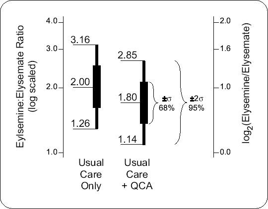
Based on the Jamkanian study reviewed above, the investigators speculate that the median EER4 for the usual care only arm is 2.0. See Figure 10.4. Two scenarios for the QCA arm are considered, a 10% decrease in EER4 (2.0 versus 1.8; as per Figure 10.4) and a 15% decrease (2.0 versus 1.7). Assuming that log2(EER4) has a Normal transformation, EER4 medians of 2.0 versus 1.8 (or 1.7) become log2(EER4) means of 1.00 versus 0.85 (or 0.77).
Making conjectures for the spread is a knotty problem, and the values chosen have critical influence on the sample-size analysis. Dr. Gooden usually takes a pragmatic approach based on the fact that, for a Normal distribution, the inter-95% range spans about 4 standard deviations. Thus, when the outcome variable is Normal, it is sufficient to estimate or guesstimate the range of the middle 95% of the infinite data set for a group and divide by 4 to set the scenario for the standard deviation.
Here, Dr. Gooden takes log(EER4) to be Normal, i.e. EER4 is logNormal, so the process is a bit more complex. Let EER40.025 and EER40.975 be the 2.5% and 97.5% quantiles of a distribution of EER4 values. With respect to log2(EER4) values, the approximate standard deviation is
Define RS95 = EER40.975/EER40.025 to be the inter-95% relative spread of EER4. For the Jamkatnian study, these were 3.04/1.10 = 2.76 and 3.28/1.50 = 2.18. To be conservative, Dr. Capote sets RS95 to be either 2.5 (as per Figure 10.4 or 3.0. Both arms are assumed to have the same relative spread. These give values for σ of log2(2.5)/4 = 0.33 and log2(3.0)/4 = 0.40.
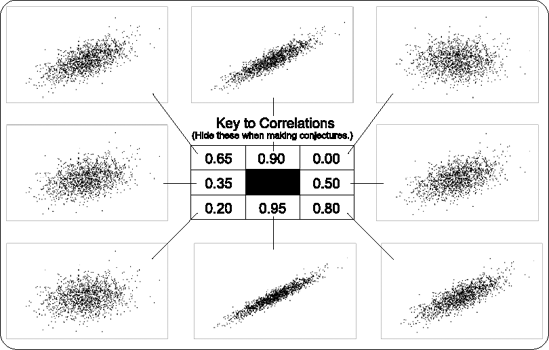
Now Dr. Gooden needs to have the team decide how strongly the three baseline covariates are correlated to log2(EER4). Technically, this correlation is the partial multiple correlation, R, of X1 = log2(EER0), X2 = plasma lacate, and X3 = log2(parasitemia) with Y = log2(EER4), controlling for treatment group, but this terminology not likely to be well understood by the CHI team. Is there any existing data on this? Not for children infected with malaria. So, Gooden asks Dr. Capote's group to imagine that some baseline index is computed by taking a linear combination of the three covariates (b1X1 + b2X2 + b3X3) in such a way that this index is maximally correlated with log2(EER4) within the two treatment groups. Dr. Gooden needs to know what R might be in the infinite dataset, but she does not simply ask them this directly, because few investigators have good understandings about what a given correlation value, say ρ = 0.30, conveys. Instead, she shows them a version of Figure 10.5 that has the values of the correlations covered from view.
The strongest correlation is most likely to be between log2(EER0) and log2(EER4). The team agrees and suspects that this is at least ρ = 0.20, even if the malaria and the treatments have a substantial impact on the metabolic pathways affecting EER. Using plasma lactate and parasitemia to also predict log2(EER4) can only increase R. Looking at the scatterplots in Figure 10.5, the team agrees that R is, conservatively, between 0.20 and 0.50.
Figure 10-5. Scatterplots showing eight degrees of correlation. The order of presentation is unsystematic to aid in eliciting more careful conjectures.
Finally, Dr. Capote wants a minimal risk of committing a Type I or Type II error for this question, so he would like to keep both α and β levels below 0.05. We will investigate the crucial error rates, α* and β*, later.
10.7.1.5. Classical Power Analysis
In order for SAS to compute the powers for this problem, two programming steps are necessary. First, Program 10.5 creates an "exemplary' data set that conforms to the conjectured infinite data set.
Example 10-5. Build and print an exemplary dataset
data EER;
  group = "UCO";
    CellWgt = 1;
    meanlog2EER_a = log2(2.0);
    meanlog2EER_b = log2(2.0);
    output;
  group = "QCA";
    CellWgt = 2;
    meanlog2EER_a = log2(1.8);
    meanlog2EER_b = log2(1.7);
    output;
  run;

proc print data=EER;
run; |
The PROC PRINT output shows that there are only two exemplary cases in the dataset, one to specify the UCO group and the other to specify the QCA group.
Example. Output from Program 10.5
Obs group CellWgt meanlog2EER_a meanlog2EER_b 1 UCO 1 1.00000 1.00000 2 QCA 2 0.84800 0.76553 |
Secondly, Program 10.6 analyzes the exemplary data set using PROC GLMPOWER.
Example 10-6. Use PROC GLMPOWER to see range of Ntotal values
proc GLMpower data=EER;
  ODS output output=EER_Ntotals;
  class group;
  model meanlog2EER_a meanlog2EER_b = group;
  weight CellWgt;
  power
    StdDev = 0.33 0.40  /* log2(2.5)/4 and log2(3.0)/4  */
    Ncovariates = 3
    CorrXY = .2 .35 .50
    alpha = .01 .05
    power = 0.95 0.99
    Ntotal = .;
run; |
Lastly, Program 10.7 summarizes the Ntotal values in a basic, but effective manner (Output 10.7). Again, more sophisticated methods are possible.
Example 10-7. Table the Ntotal values
* Augment GLMPOWER output to facilitate tabling ;
data EER_Ntotals; set EER_Ntotals;
  if dependent = "meanlog2EER_a" then EEratio = "2.0 vs 1.8";
  if dependent = "meanlog2EER_b" then EEratio = "2.0 vs 1.7";;
  if UnadjStdDev = 0.33 then RelSpread95 = 2.5;
  if UnadjStdDev = 0.40 then RelSpread95 = 3.0;
  run;

proc tabulate data=EER_Ntotals format=5.0 order=data;
  format Alpha 4.3 RelSpread95 3.1;
  class EEratio alpha RelSpread95 CorrXY NominalPower;
  var Ntotal;
  table
    EEratio="EE Ratios: "
      * alpha="Alpha"
      * NominalPower="Power",
    RelSpread95="95% Relative Spread"
      * CorrXY="Partial R for Covariates"
      * Ntotal=""*mean=" "
    /rtspace=35;
run; |
Example. Output from Program 10.7
----------------------------------------------------------------------- | | 95% Relative Spread | | |-----------------------------------| | | 2.5 | 3.0 | | |-----------------+-----------------| | | Partial R for | Partial R for | | | Covariates | Covariates | | |-----------------+-----------------| | |0.20 |0.35 |0.50 |0.20 |0.35 |0.50 | |---------------------------------+-----+-----+-----+-----+-----+-----| |EE Ratios:|Alpha |Power | | | | | | | |----------+----------+-----------| | | | | | | |2.0 vs 1.8|.010 |0.95 | 369| 336| 288| 537| 492| 420| | | |-----------+-----+-----+-----+-----+-----+-----| | | |0.99 | 495| 453| 387| 723| 663| 567| | |----------+-----------+-----+-----+-----+-----+-----+-----| | |.050 |0.95 | 267| 246| 210| 393| 360| 306| | | |-----------+-----+-----+-----+-----+-----+-----| | | |0.99 | 378| 345| 297| 552| 507| 432| |----------+----------+-----------+-----+-----+-----+-----+-----+-----| |2.0 vs 1.7|.010 |0.95 | 156| 144| 123| 228| 210| 180| | | |-----------+-----+-----+-----+-----+-----+-----| | | |0.99 | 210| 192| 165| 306| 282| 240| | |----------+-----------+-----+-----+-----+-----+-----+-----| | |.050 |0.95 | 114| 105| 90| 168| 153| 132| | | |-----------+-----+-----+-----+-----+-----+-----| | | |0.99 | 162| 147| 126| 234| 216| 183| ----------------------------------------------------------------------- |
Upon scanning the results in Output 10.7, Drs. Capote and Gooden decide that Ntotal = 100 + 200 may be minimally sufficient, and Gooden focuses on this by using Program 10.8.
Example 10-8. Compute and table powers at Ntotal = 300 for EER4 outcome
proc GLMpower data=EER;
  ODS output output=EER_powers;
  class group;
  model meanlog2EER_a meanlog2EER_b = group;
  weight CellWgt;
  power
    StdDev = 0.33 0.40  /* log2(2.5)/4 and log2(3.0)/4 */
    Ncovariates = 3
    CorrXY = .2 .35 .5
    alpha = .01 .05
    Ntotal = 300
    power = .;
  run;

* Augment GLMPOWER output to facilitate tabling ;
data EER_powers; set EER_powers;
  if dependent = "meanlog2EER_a" then EEratio = "2.0 vs 1.8";
  if dependent = "meanlog2EER_b" then EEratio = "2.0 vs 1.7";;
  if UnadjStdDev = 0.33 then RelSpread95 = 2.5;
  if UnadjStdDev = 0.40 then RelSpread95 = 3.0;
  if power > .999 then power999 = .999;
    else power999 = power;
  run;

proc tabulate data=EER_powers format=4.3 order=data;
  format Alpha 4.3 RelSpread95 3.1;
  class EEratio alpha RelSpread95 CorrXY Ntotal;
    var power999;
    table
      Ntotal="Total Sample Size: ",
      EEratio="EE Ratios: "
        * alpha="Alpha",
      RelSpread95="95% Relative Spread"
        * CorrXY="Partial R for Covariates"
        * power999=""*mean=" "
  /rtspace=35;
run; |
Output 10.8 shows that only in the most pessimistic scenario does the power wane a little below 0.90 using Ntotal = 300 and α = 0.05, and the mid-range scenarios even have substantial power at α = 0.01. Furthermore, with Ntotal = 300, the assay costs associated with this aim will run about 300 × US$120 = US$36000, which is deemed practical. The CHI team still wants to assess the crucial Type I and Type II error rates.
Example. Output from Program 10.8
Total Sample Size: 300 ----------------------------------------------------------------- | | 95% Relative Spread | | |-----------------------------| | | 2.5 | 3.0 | | |--------------+--------------| | |Partial R for |Partial R for | | | Covariates | Covariates | | |--------------+--------------| | |0.20|0.35|0.50|0.20|0.35|0.50| |---------------------------------+----+----+----+----+----+----| |EE Ratios: |Alpha | | | | | | | |----------------+----------------| | | | | | | |2.0 vs 1.8 |.010 |.893|.922|.959|.717|.764|.838| | |----------------+----+----+----+----+----+----| | |.050 |.969|.979|.991|.884|.910|.946| |----------------+----------------+----+----+----+----+----+----| |2.0 vs 1.7 |.010 |.999|.999|.999|.989|.994|.998| | |----------------+----+----+----+----+----+----| | |.050 |.999|.999|.999|.998|.999|.999| ----------------------------------------------------------------- |
10.7.2. Crucial Type I and Type II Error Rates
Based on the current state of knowledge reviewed above, Dr. Capote's team's believes that while this hypothesis is important to investigate seriously, there is only a 20-30% chance that QCA affects EER. Accordingly, Dr. Gooden uses Program 10.9 to convert the results given in Output 10.8 to the crucial error rates.
Example 10-9. Compute and table crucial error rates for EER4 outcome
%CrucialRates (   PriorPNullFalse= .20 .30,
                  Powers = EER_powers,
                  CrucialErrRates = EERCrucRates )

proc tabulate data=EERCrucRates format=4.3 order=data;
title3 "Crucial Error Rates for EER Outcome";
  format Alpha 4.3 RelSpread95 3.1;
  class TypeError gamma EEratio alpha RelSpread95 CorrXY Ntotal;
  var CrucialRate;
  table
    Ntotal="Total N: ",
    EEratio="EE Ratios: "
      * RelSpread95="95% Relative Spread"
      * CorrXY="Partial R for Covariates",
    alpha="Alpha"
      * gamma="PriorP[Null False]"
      * TypeError="Crucial Error Rate"
      * CrucialRate=""*mean=" "
    / rtspace = 32;
run; |
Example. Output from Program 10.9
Total N: 300 ------------------------------------------------------------------------ | | Alpha | | |---------------------------------------| | | .010 | .050 | | |-------------------+-------------------| | |PriorP[Null False] |PriorP[Null False] | | |-------------------+-------------------| | | 0.2 | 0.3 | 0.2 | 0.3 | | |---------+---------+---------+---------| | | Crucial | Crucial | Crucial | Crucial | | | Error | Error | Error | Error | | | Rate | Rate | Rate | Rate | | |---------+---------+---------+---------| | |Type|Type|Type|Type|Type|Type|Type|Type| | | I | II | I | II | I | II | I | II | |------------------------------+----+----+----+----+----+----+----+----| |EE |95% |Partial R | | | | | | | | | |Ratios: |Relative |for | | | | | | | | | |---------|Spread |Covariates| | | | | | | | | |2.0 vs |---------+----------| | | | | | | | | |1.8 |2.5 |0.20 |.043|.026|.025|.044|.171|.008|.107|.014| | | |----------+----+----+----+----+----+----+----+----| | | |0.35 |.042|.019|.025|.033|.170|.005|.106|.009| | | |----------+----+----+----+----+----+----+----+----| | | |0.50 |.040|.010|.024|.017|.168|.002|.105|.004| | |---------+----------+----+----+----+----+----+----+----+----| | |3.0 |0.20 |.053|.067|.032|.109|.184|.030|.117|.050| | | |----------+----+----+----+----+----+----+----+----| | | |0.35 |.050|.056|.030|.093|.180|.023|.114|.039| | | |----------+----+----+----+----+----+----+----+----| | | |0.50 |.046|.039|.027|.065|.174|.014|.110|.024| |---------+---------+----------+----+----+----+----+----+----+----+----| |2.0 vs |2.5 |0.20 |.038|.000|.023|.000|.167|.000|.104|.000| |1.7 | |----------+----+----+----+----+----+----+----+----| | | |0.35 |.038|.000|.023|.000|.167|.000|.104|.000| | | |----------+----+----+----+----+----+----+----+----| | | |0.50 |.038|.000|.023|.000|.167|.000|.104|.000| | |---------+----------+----+----+----+----+----+----+----+----| | |3.0 |0.20 |.039|.003|.023|.005|.167|.000|.105|.001| | | |----------+----+----+----+----+----+----+----+----| | | |0.35 |.039|.002|.023|.003|.167|.000|.105|.000| | | |----------+----+----+----+----+----+----+----+----| | | |0.50 |.039|.000|.023|.001|.167|.000|.104|.000| ------------------------------------------------------------------------ |
Dr. Capote likes what he sees here using α = 0.01, because almost all the α* and β* values are less than 0.05. The CHI team decides to use α = 0.01 and Ntotal = 100 + 200 subjects for the EER component of this trial.
10.7.3. Using Baseline Covariates in Randomized Studies
What are the consequences of failing to use helpful baseline covariates when comparing adjusted group means in randomized designs? What are the consequences of using worthless baseline covariates—those that have no value whatsoever in predicting the outcome (Y)? Researchers face this question because each additional covariate requires another parameter to be estimated, and this decreases by 1 the degrees of freedom for error for the F test of the group differences.
The question is easily addressed and the answer surprises many. Consider the power values displayed in Table 10.5, were obtained by modifying the PROC GLMPOWER code in Program 10.8. Here, we limit our focus to the case with EER medians of 2.0 versus 1.8, with a 95% relative spread of 2.5, Ntotal = 300 and α = 0.01. On the other hand, we consider several more values for R (SAS Code: CorrXY 0 .20 .35 .50 .70) and three possible values for the number of covariates (SAS Code: Ncovariates = 0 3 50).
| Number of covariates used | Multiple partial correlation (R) | ||||
|---|---|---|---|---|---|
| 0.00 | 0.20 | 0.35 | 0.50 | 0.70 | |
| 0 | .878 | .878 | .878 | .878 | .878 |
| 3 | .878 | .893 | .922 | .959 | .996 |
| 50 | .877 | .892 | .921 | .959 | .996 |
The point here is obvious. In a randomized design, there is virtually no cost associated with using worthless baseline covariates, because they are uncorrelated with the group assignment. The only cost is that the nominal null F distributions change, but in this case, the 0.01 critical values for F(1, 298) and F(1, 248) are 6.72 and 6.74, respectively, which are virtually equal. On the other hand, there is a high cost to be paid by not using baseline covariates that have some value in predicting the outcome. This concept holds for both continuous and categorical outcomes.